Time Series Smoothing
In time series analysis, data often contains a high degree of noise—random, short-term fluctuations that can obscure the underlying patterns. Smoothing is the process of removing this noise to reveal the true trend, seasonality, or cyclical components.
The goal of smoothing is to create a new, less volatile time series that is easier to analyze and forecast. Here, we’ll cover the most common techniques used for this purpose.
Moving Average
The moving average is the simplest and most intuitive smoothing technique. It works by creating a new series where each value is the average of a specific number of preceding data points. This process “irons out” the noise by averaging out random variations.
\[\hat{y_t} = \frac{1}{k} \sum_{i=0}^{k-1} y_{t-0}\]Here $k$ is the number of data points included in the average (the window size).
This type of smoothing is simple to understand and compute; however, it can lag behind the original data heavily and may be impacted by large spikes.
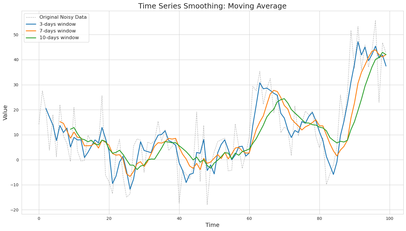
As can be seen, the larger the window, the smoother the resulting series is. However, it also becomes the most lagging of all and requires the biggest number of data points upfront. On the other hand, a shorter window may not produce the desired level of smoothing.
Exponential Smoothing
This is a more sophisticated method that gives more weight to recent observations, making the smoothed series more responsive to recent changes. It applies a “smoothing factor” ($\alpha$), a weight that decreases exponentially for older data points.
\[\hat{y_t} = \alpha y_t + (1-\alpha) \hat{y_{t-1}}\]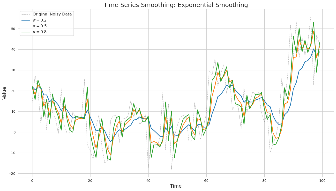
The choice of the $\alpha$ value can significantly impact the result. The higher its value, the less smooth the resulting time series will be.
Similar to the moving average, this algorithm also suffers from lagging behind the original trends in the data.
Kalman Filter
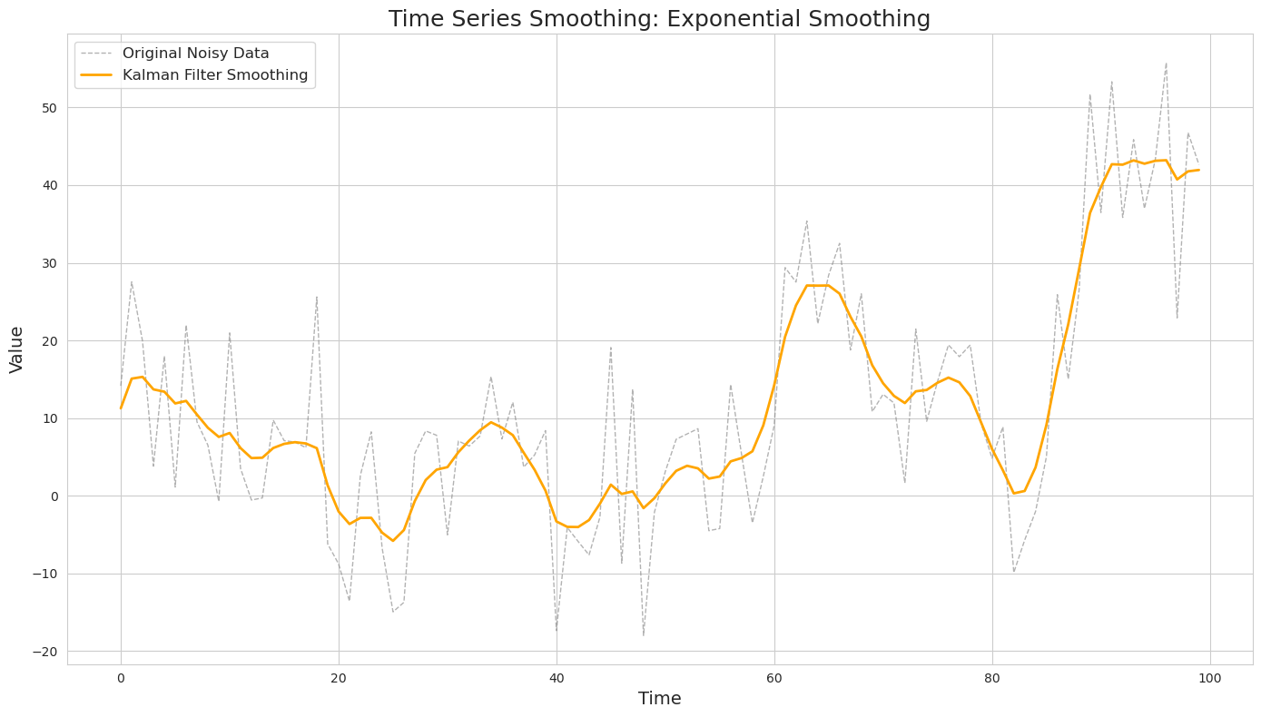
The Kalman filter is a powerful and highly advanced technique, particularly useful in signal processing and engineering. It’s an iterative, two-step process that provides an optimal estimate of a system’s state from a series of noisy measurements.
The filter operates on the principle that the system’s true state can be estimated more accurately by combining a prediction based on a mathematical model and a noisy measurement.
The Kalman filter’s power comes from its ability to handle multiple variables at once and its capacity to provide an optimal estimate in real-time. Below is an example of the application of a Kalman filter to the same simulated dataset as the one used for moving average and exponential smoothing.
Two-Step Process
Prediction: The filter predicts the next state of the system based on a mathematical model. It also calculates the uncertainty of that prediction and the system’s dynamics.
Update: When a new measurement arrives, the filter updates the predicted state by giving more weight to either the prediction or the new measurement, depending on their respective uncertainties.
The Core Equations
The state of the system at any time $k$ is defined by a vector $x_k$ which consists of various factors that determine this state (e.g., velocity, temperature, position, or any other characteristic of interest). This true vector is unknown.
According to Kalman filter, the true state at time $k$ evolves from time $k-1$ according to this formula:
\[x_k = F_k x_{k-1} B_k u_k + w_k\]Here
- $F_k$ is a state transition model.
- $u_k$ is a control input vector (if present) that represents some external influence.
- $B_k$ is a control input model which is applied to the control input vector.
- $w_k$ is the process noise, which is assumed to be drawn from a multivariate normal distirbution centered at 0 with covariance matrix $Q_k$
Because the system model’s accuracy can fluctuate over time, $F$ is actually an approximation, and $Q$ serves to represent this uncertainty.
The Kalman filter also uses the covariance matrix $P$ of the elements from $x_k$ to better predict the state. For example, the state could be a vector with two elements: position and velocity. These two elements are correlated, so knowing one allows for a better prediction of the other.
At the same time, we have a measurement of the true state:
\[z_k = H_k x_k + v_k\]where
- $H_k$ is the measurement model, which maps the true state space into the observed state space. This could be the case for different scales and units of measurement.
- $v_k$ s the measurement noise, which is assumed to be zero mean Gaussian white noise with a covariance $R_k$.
What the algorithm is trying to find is an overlap of the two regions: the prediction with its area of uncertainty and the measurement with its own area of uncertainty. The resulting region will produce a value that is more precise with respect to the true state than either of its two components.
The distributions of both $x$ and $z$ are Gaussian. The mean and variance of the joint distribution are calculated as follows:
\[\mu ' = \mu_{0} + \frac{\sigma_{0}^{2} (\mu_{1} - \mu_{0})}{\sigma_{0}^{2} + \sigma_{1}^{2}}\] \[{\sigma}'^{2} = \sigma_{0}^{2} - \frac{\sigma_{0}^{4}}{\sigma_{0}^{2} + \sigma_{1}^{2}}\]By making a small substitution, we get this:
\[k = \frac{\sigma_{0}^{2}}{\sigma_{0}^{2} + \sigma_{1}^{2}}\] \[\mu ' = \mu_{0} +k(\mu_{1} - \mu_{0})\] \[{\sigma}'^{2} = \sigma_{0}^{2} - k \sigma_{0}^{2}\]In matrix notation, $K$ is known as the Kalman gain and can be written as this:
\[K = \Sigma_0 (\Sigma_0 + \Sigma_1)^{-1}\]Application of this Kalman gain to the model leads to the minimization of the errors from the joint distribution of predictions and measurements.
With respect to the Kalman Filter algorithm, it is important to specify a sensible guess for the initial state (our first estimate) in order to advance it forward. We also have to specify the variance of the process noise ($Q$), and the variance of the measument noise ($R$).
Now, using this, at each time step $k$ the Kalman filter applies the following equations in its iterative process:
Prediction Step:
- Project the state ahead:
- Project the error covariance ahead:
Here $\hat{x}{k∣k−1}$ and $\hat{x}{k∣k}$ are predicted and updated state vectors.
Update Step:
- Calculate pre-fit measurement residual (innovation):
- Calculate pre-fit residual covariance:
- Compute the Kalman gain:
- Update the state estimate:
- Update the prediction covariance:
- Calculate the measurement post-fit residual:
At each step, the estimated covariance $P$ (the estimate’s uncertainty) will be smaller. If $R$ (the measurement uncertainty) is large, the Kalman gain would be lower, and thus the convergence of $P$ will be slower.
Fixed-interval smoothers
A fixed-interval smoother is a powerful technique that provides the most accurate estimate for a time series after you have collected all of your data, from start to finish.
The standard Kalman filter, as we’ve discussed, is a real-time, one-pass algorithm. It produces the best estimate of the current state based on all past and current measurements. A smoother, on the other hand, runs a second, backward pass through the data to refine the estimates for all previous time points, using information from the future. The Rauch-Tung-Striebel (RTS) Smoother is a well-known example of a fixed-interval smoother.
Here is how RTS Smoother works:
-
During its forward pass the Kalman Filter saves the history of its predicted and updated state estimates: $\hat{x}_{k\mid k-1}$ and $\hat{x}_{k∣k}$, as well as covariances $P_{k\mid k−1}$ and $P_{k\mid k}$.
-
After all forwards passes are completed, the point estimates are processed in a reversed order by apllying these equations:
- Calculating the smoother gain matrix ($G_k$): This gain determines how much to weigh the new information from the subsequent state.
- Updating the smoothed state estimate. This is the final, optimal state estimate at time $k$, using all data up to time $N$.
- Updating the smoothed covariance estimate. This represents the reduced uncertainty of the final smoothed estimate.
Estimating parameters
The Kalman filter requires the process noise covariance ($Q$) and the measurement noise covariance ($R$) to be known beforehand. The Expectation Maximization algorithm (EM) provides a perfect solution for this problem by treating the unknown states as latent variables and the unknown covariances as the parameters we need to estimate.
The EM algorithm for the Kalman filter (often called the EM-Kalman smoother) works as follows:
The E-Step: The Kalman Smoother Pass
The E-step of the EM algorithm is where the Kalman filter and the RTS smoother do their work. Here the E-step essentially calculates the necessary statistics from the data, such as the smoothed mean and covariance of the state and measurement residuals, which will be used in the next step.
The M-Step: Updating the Parameters
The formulas for the new estimates ($Q$ and $R$) are derived from the principle of maximum likelihood. The goal is to find values for Q and R that best explain the discrepancies (residuals) we observed between our model and our data.
\[\hat{Q} = \frac{1}{N} \sum_{k=1}^{N}[(\hat{x}_{k∣N} - F_k \hat{x}_{k-1∣N})(\hat{x}_{k∣N} - F_k \hat{x}_{k-1∣N})^{T} + P_{k∣N} - F_k P_{k-1∣N}F_k^{T}]\]This formula effectively averages two components: the squared residuals, and the uncertainty in the state transitions over the entire time series.
The squared residual term is a measure of the squared error. It calculates the difference between the most accurate estimate of the state at time $k$ (the smoothed state $\hat{x}_{k \mid N}$), and the one-step prediction of that state $F_k \hat{x}_{k-1 \mid N}$. This term tells us how much our dynamics model was “wrong” at each step.
The covariance term accounts for the uncertainty in our estimates. It subtracts the uncertainty of the predicted state from the uncertainty of the smoothed state. This ensures that the updated value for $Q$ reflects the inherent randomness of the system’s evolution, not just the errors from our estimates.
\[\hat{R} = \frac{1}{N} \sum_{k=1}^{N}[(z_k - H_k \hat{x}_{k∣N})(z_k - H_k \hat{x}_{k∣N})^{T} + H_k P_{k∣N} H_k^{T}]\]This formula averages the squared residuals between the actual measurements and the smoothed state projections, accounting for the uncertainty in those projections. Here the covariance term $H_k P_{k∣N} H_k^{T}$ accounts for the uncertainty in the smoothed state as it’s projected into the measurement space. This ensures our estimate of $R$ isn’t just a measure of the raw difference but an honest estimate of the noise.
The algorithm repeats these two steps—E-step (smooth) and M-step (update)—until the estimates for $Q$ and $R$ no longer change significantly.