Time Series Analysis

Time series analysis is a specialized field of statistics that focuses on data points collected over time. From daily stock prices and hourly temperature readings to monthly sales figures, time series data is distinct because the order of observations matters. Unlike traditional regression, where data points are assumed to be independent, a key feature of time series is that each observation is often influenced by what came before it. This dependence is the very essence of a time series.

Foundational Concepts

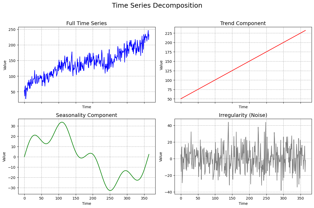
Before diving into the models, it is essential to understand the fundamental components of a time series:

• Trend: The long-term, underlying movement in the data (e.g., a gradual increase or decrease over many years).
• Seasonality: A predictable, repeating pattern or cycle that occurs over a fixed period, such as daily, weekly, or yearly cycles (e.g., retail sales peaking every December).
• Cyclicality: Patterns that are not of a fixed period and are often associated with broader economic cycles (e.g., recessions and booms).
• Noise: Random, unpredictable fluctuations in the data that are not explained by the other components.

The Role of Regression

Many time series models are a direct application of regression principles. A key concept is Autoregression (AR), where the value of a variable at a given time is regressed on its own past values. This method effectively uses prior data points as independent variables to forecast future values.

Core Methods for Analysis and Forecasting

The goal of time series analysis is to understand the past to predict the future. The following methods are widely used to model time series data:

Smoothing and Simple Models

These methods are often a good starting point for forecasting. They are used to remove noise and reveal the underlying patterns in the data. Exponential smoothing is one such technique that gives more weight to recent observations and is highly effective for short-term forecasting. For a detailed look at the smoothing techniques, see this article.

ARIMA Models

ARIMA (Autoregressive Integrated Moving Average) is a powerful class of models that combine autoregression with two other key components:

• Integration (I): This involves differencing the data to make it stationary, which means removing trends and seasonality.

• Moving Average (MA): This accounts for the relationship between an observation and a lagged residual error.

ARIMA models are a sophisticated way to handle complex time series data. To learn more about them, see the dedicated article on ARIMA Models.

Advanced and Specialized Models

While ARIMA and exponential smoothing are powerful, some real-world problems require more specialized approaches.

The Kalman Filter: This is a crucial algorithm used for state estimation. It’s particularly useful for filtering out noise from a time series and making predictions for a system where the state is not directly observable. It’s the underlying technology for many applications, including GPS navigation, where it estimates a vehicle’s position based on noisy sensor readings.

Vector Autoregression (VAR): All the models above are for a single time series. VAR extends the autoregression concept to multiple interdependent time series. It’s used to analyze the dynamic relationship between several variables, such as the relationship between inflation, interest rates, and GDP.

Other Models: The field is continuously evolving with new models designed for specific problems. These include models like Prophet (used for business forecasting with complex seasonal patterns and holidays) and GARCH (used for modeling volatility in financial time series).