Exponential smoothing models

In this article we shall make a breakdown of the exponential smoothing models which are used in time series forecasting.

• Simple exponential smoothing model
• Exponential smoothing with trend
• Exponential smoothing with trend and seasonality
• State space models with additive and multiplicative errors

Simple exponential smoothing model

Similarly to ARIMA models the idea upon which the exponential smoothing models are built is that the most recent observations contribute to the currently observed values of a series. Unlike ARIMA models however they do not require the time series to be stationary, and the weights with which the recent observation influences the current one decay exponentially, hence the name.

This is how the relationship between the observations can be expressed:

\[\hat{y}_{t+1|t}=\alpha y_{t} + (1-\alpha) \alpha y_{t-1} + (1-\alpha)^{2} \alpha y_{t-2} + \cdots\]

Here $\alpha$ is the parameter which controls the strength of the relationship between the currently observed value and the values at different lags: the higher the value of $\alpha$ - the bigger weight is placed on the most recent observation, and the quicker the weight of each further previous observation decays. In other words the most recent observation has weight equal to $\alpha$, and all other observations combined have weight $(1-\alpha)$ with respect to $y_{t+1}$. At the same time $y_t$ is also defined via exponential smoothing, and it places weight $\alpha$ to $y_{t-1}$ and weight $(1-\alpha)$ to all other previous observations. The same is true for all other previous observations which explains the final form of the equation above.

Notice that there is no explicit error term because it is believed to be incorporated within the past observed values. The model makes a forecast based on the previous disturbance so for now it has only a single term - the level component which is the weighted average of the observed value at $t$ and of the forecasted value at $t$ given the value at $t-1$:

\[\ell_{t} = \alpha y_{t} + (1 - \alpha)\ell_{t-1}\]

Let’s introduce the component form of the forecast equation above which for now will include only the level component.

\[\hat{y}_{t+h|t} = \ell_{t}\]

Here $h$ is the step size for the forecast so the given expression is the forecast for the point $y_{t+h}$ given the observed values up until $y_t$.

The component form is a useful representation of the exponential smoothing model because it can later be extended to include the trend and seasonal components (and this is where the step size $h$ will actually start to matter).

Back to top ↑

Exponential smoothing with trend

Also known as Holt’s linear trend method, it utilizes the component form of the forecast equation, and contains two terms: the level and the trend components.

\[\hat{y}_{t+h|t} = \ell_{t} + hb_t\]

where $b_t$ is the estimate of the trend at point $t$:

\[b_t = \beta^*(\ell_{t} - \ell_{t-1}) + (1 -\beta^*)b_{t-1}\]

and the level component accommodates for the previously estimated trend component:

\[\ell_{t} = \alpha y_{t} + (1 - \alpha)(\ell_{t-1}+b_{t-1})\]

Notice how the component form of the forecast equation resembles the simple linear regression where the level component is the intercept, and the forecast is a linear function of the step size $h$.

Since the same trend into the future is hardly realistic, a dampening factor $\phi$ was introduced into the model which lessens the effect of the trend for increasing forecasting windows.

\[\begin{align*} \hat{y}_{t+h|t} &= \ell_{t} + (\phi+\phi^2 + \dots + \phi^{h})b_{t} \\ \ell_{t} &= \alpha y_{t} + (1 - \alpha)(\ell_{t-1} + \phi b_{t-1})\\ b_{t} &= \beta^*(\ell_{t} - \ell_{t-1}) + (1 -\beta^*)\phi b_{t-1}. \end{align*}\]

$\phi$ can be set somewhere between 0 and 1. If it’s equal to 1 then the model will not include the trend dampening.

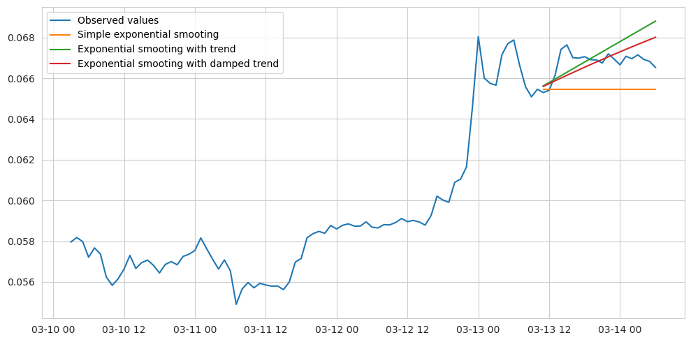
Below we can see an example of forecasting with exponential smoothing having with and and without the trend component.

Back to top ↑

Exponential smoothing with trend and seasonality

This type of model is known as Holt-Winters’ seasonal method, and it adds the seasonal component to the equation. There are actually two variants of this model: with the additive and with the multiplicative seasonal component.

The additive model is built like this:

\[\begin{align*} \hat{y}_{t+h|t} &= \ell_{t} + hb_{t} + s_{t+h-m(k+1)} \\ \ell_{t} &= \alpha(y_{t} - s_{t-m}) + (1 - \alpha)(\ell_{t-1} + b_{t-1})\\ b_{t} &= \beta^*(\ell_{t} - \ell_{t-1}) + (1 - \beta^*)b_{t-1}\\ s_{t} &= \gamma (y_{t}-\ell_{t-1}-b_{t-1}) + (1-\gamma)s_{t-m}, \end{align*}\]

Here $m$ is the number of observations for a full cycle, for example 12 in case of monthly data. $k$ is the integer part of the expression $(h-1)/m$ which is meant to ensure that the estimate of the seasonal component is taken from the latest observed cycle.

The multiplicative model is built like this:

\[\begin{align*} \hat{y}_{t+h|t} &= (\ell_{t} + hb_{t})s_{t+h-m(k+1)} \\ \ell_{t} &= \alpha \frac{y_{t}}{s_{t-m}} + (1 - \alpha)(\ell_{t-1} + b_{t-1})\\ b_{t} &= \beta^*(\ell_{t}-\ell_{t-1}) + (1 - \beta^*)b_{t-1} \\ s_{t} &= \gamma \frac{y_{t}}{(\ell_{t-1} + b_{t-1})} + (1 - \gamma)s_{t-m} \end{align*}\]

The difference between the two models is that with the additive one the level of the seasonal component is expected to be the same from cycle to cycle, while in the multiplicative model it changes with the level of the series. Back to top ↑

State space models with additive and multiplicative errors

The state space models utilize the approach of evolutionary updating the parameters with each new observation. When a new observation comes out, the error is measured by comparing the observed value with the previously predicted one. For example the equation for level component in the simple exponential smoothing model could be rearranged to look like this:

\[\begin{align*} \ell_{t} &= \ell_{t-1}+\alpha( y_{t}-\ell_{t-1})\\ &= \ell_{t-1}+\alpha \varepsilon_{t} \end{align*}\]

where $\varepsilon_{t}$ is the measured error at point $t$.

The level parameter here is the state which is adjusted by the measured error damped by the smoothing parameter $\alpha$. The state space models do this type of updating for a space of states (level, trend, seasonality) simultaneously with each new observation, hence the name. The smoothing parameters are optimized so that the total error along the whole series of observations is minimized.

The error representation above is known as an additive error model. The alternative is the multiplicative error model, where the error is represented as a relative difference instead of the absolute one.

\[\varepsilon_t = \frac{y_t-\hat{y}_{t|t-1}}{\hat{y}_{t|t-1}}\]

which naturally implies a different form of the state space equations.

By introducing the error term into the equation, the state space models are capable of generating not only the point estimates but also the confidence intervals (under the assumption that the errors are independent and normally distributed). Back to top ↑