Change point analysis

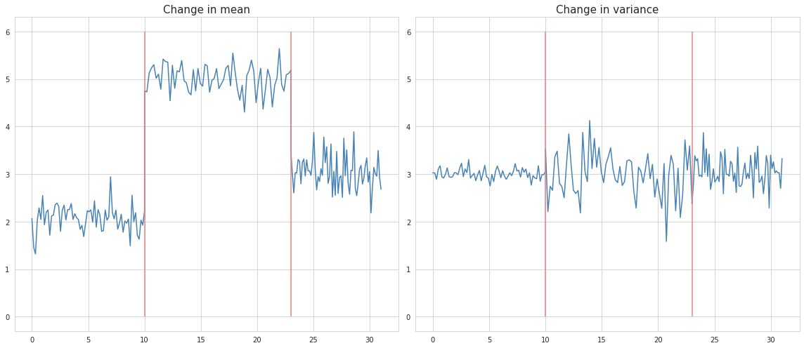
Change point analysis is basically used for determining whether and where an ordered series of values (usually time series) changed their behaviour. The change of behaviour may include the change in mean, variance or both.

In the real life situations however, the recognition of the change points by eyeballing is not as simple as it sounds, especially if the time series contain spikes, trends and seasonality. Other than that, usually it is desired to be able to detect the break points automatically, without having to look at the charts.

There are two types of change point analysis: offline and online. Offline methods analyze the whole series at once, and they are more accurate in detection of the change points. On the contrary, the online methods are used for the quickest detection of the change points in the newly arrived datapoints (for example in streaming signals). Another application of online methods is anomaly detection.

Offline change point analysis

The offline change point analysis can be viewed as a segmentation task where the signal should be split into multiple non-overlapping pieces according to some cost function minimization:

     $V(\tau, y ) = \sum_{k=0}^K c(y_{t_{k}})$

where $y$ is the signal, $\tau$ represents the number of splits, and $c(y)$ is a piecewise cost function.

In the literature, the actual break points are denoted by ${T}^{\ast} = \{ \tau_{1}^{\ast}, …, \tau_{K}^{\ast} \}$, while the estimated ones as ${\hat{T}}=\{\hat{\tau_{1}}, …, \hat{\tau_{K}}\}$.

Offline change point detection models have three components which distinguish them one from another. These are:

• Cost function, which is a measure of homogenity: the lower its value - the more homogeneous are the points. The cost function is selected according to the type of changes which need to be detected.
• Search method of cost function optimization, that is way how the parameters of the the cost function are determined.
• Constraint (on the number of change points). If the number of changes is not known, a constraint (or penalty, or artificial noise) is added to the cost function in order to prevent overfitting. The volume of penalizations depends on the magnitude of the expected changes: the greater the penalty - the less certain the model is on the existance of a break point at a certain spot. This is why only the most significant changes will be detected.

Evaluation metrics

In order to evaluate the robustness of a model Hausdorf metric is used, which equals to the worst error made by the model that produced ${\hat{T}}$, and is expressed in number of samples.

The accuracy can be measured by the Rand index which represents the number of times when a certain point belongs to the same structural segment according the model, and to the ground truth. This metric is normalized so that it assumes values between 0 and 1.

The precision of the model can be determined as the proportion of determined change points which are true change points, while the recall is the number of true change points which are correctly determined. In addition, some user-defined margin ($M >0$) can be set where the break point is considered to be correctly determined. It is recommended to set the margin smaller than the minimum between the two true break points. With regard to the precision and recall, the $F1$ score is defined as a harmonic mean between these metrics:

     $\Delta_{F1}({T}^{\ast}, \hat{T}) = 2 \times \frac{Prec({T}^{\ast}, \hat{T}) \times Rec({T}^{\ast}, \hat{T})}{Prec({T}^{\ast}, \hat{T}) + Rec({T}^{\ast}, \hat{T})}$

The $F1$ score assumes values between 1 and 0, whereas the greater its value - the better the model.