Parametric Survival Models
Parametric survival models assume that survival times follow a known probability distribution. Unlike non-parametric methods (Kaplan–Meier) or semi-parametric ones (Cox PH), these models specify the exact form of the hazard function $h(t)$.
This yields interpretable parameters, smooth curves, and the ability to predict beyond the observed data range.
Model Framework
A parametric survival model defines a probability density $f(t;\theta)$ and cumulative distribution $F(t;\theta)$ with parameters $\theta$ of the hazard event. The survival and hazard functions are expressed as follows:
\[S(t) = 1 - F(t;\theta)\] \[h(t) = \frac{f(t; \theta)}{S(t; \theta)}\]With covariates $X$, the hazard or survival time is related through a regression structure, typically via one of two formulations described below.
Proportional Hazards (PH) Form
\[h(t|X) = h_0(t) \exp(\beta^T X)\]Same structure as the Cox model, but here $h_0(t)$ is known (e.g., exponential or Weibull).
Accelerated Failure Time (AFT) Form
A subclass of parametric survival models focusing on time scaling rather than hazard scaling. Equivalent to log-linear regression on $T$:
\[\log(T_i) = \mu + \beta^T X_i + \sigma \varepsilon_i\]where $\varepsilon_i$ follows a known distribution (e.g., extreme value, logistic, normal). This model describes how covariates accelerate or decelerate the event time.
For example, if $\exp (\beta_j) = 1.5$ then it would mean that the expected survival time is 1.5 longer for a one-unit increase in $X_j$
Common Parametric Distributions
| Distribution | Survival function $S(t)$ | Hazard function $h(t)$ | Hazard function shape | Interpretation |
|---|---|---|---|---|
| Exponential | $e^{-\lambda t}$ | $\lambda$ | Constant | Memoryless process |
| Weibull | $e^{-(\lambda t)^{k}}$ | $\lambda k(t)^{k-1}$ | increases if $k$ > 1, decreases if $k$ < 1 | Very flexible; includes exponential as $k=1$ |
| Log-Logistic | $[1+t/ \lambda^{k}]^{-1}$ | $\frac{(k/\lambda)(t/\lambda)^{k-1}}{1+t/ \lambda^{k}}$ | Unimodal | Hazard rises then falls |
| Log-Normal | $1- \Phi\left(\frac{\ln t - \mu}{\sigma} \right)$ | non-monotonic | Flexible | Useful when long right tail |
Each provides a different hazard shape, letting the analyst select based on domain knowledge or data diagnostics.
Parameter Estimation
Parameters are estimated with Maximum Likelihood Estimation:
\[\mathcal{L}(\theta) = \prod_{i=1}^n [f(t_i; \theta)]^{\delta_i} [S(t_i; \theta)]^{1-\delta_i}\]where $\delta_i = 1$ if the event occurred, 0 if censored. This formulation naturally accounts for right-censoring.
Parametric vs Semi-parametric (Cox PH) Estimator
| Feature | Cox PH | Parametric Model |
|---|---|---|
| Baseline hazard $h_0(t)$ | Unknown, estimated nonparametrically | Known functional form (Exponential, Weibull, Log-logistic, etc.) |
| Assumption strength | Weak (semi-parametric) | Strong |
| Interpretability | Relative risk (hazard ratio) | Can yield absolute predictions (mean survival time, etc.) |
| Extrapolation | Limited (data-driven) | Possible (based on assumed distribution) |
Suppose we use Weibull (parametric) model in PH form:
\[h(t|X) = \lambda k t^{k-1} e^{\beta^T X}\]Here $\lambda$ and $k$ distribution parameters controlling scale and shape. So it’s also “proportional hazards” (covariates enter multiplicatively), but unlike with Cox PH the shape of the hazard over time is fixed by the Weibull functional form.
On the other hand, the Cox model can fit a much wider range of survival patterns without assuming the exact distribution of survival times which makes it a more robust and flexible choice.
For demonstration purposes let’s fit both models to simulated data to see how they differ. The survival function from parametric Weibull distribution will take the following form
\[S(t|X) = \exp[-(\lambda t)^k e^{\beta^T X}]\]And the survival function from from Cox semi-parametric model will take this form:
\[S(t|X) = \exp[-(h_0(t) e^{\beta^T X}]\]We have a single covariate $X$ which can assume values 1 or 0.
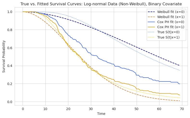
As can be seen from the example plot above, Weibull fit, unlike Cox PH, produces a smooth curve. Even though the fitted distribution is not the same as the one which generates the data, it can still be closer to it because the parameters are considering the change in time.
| On the other hand, Cox PH is also pretty close. Even if we consider the case when $X=0$ then the survival function collapses to this: $S(t | X) = \exp[-(h_0(t)]$ which becomes the average survival regardless of the actual $X$. And this is exactly what we observe on the chart. |