Kaplan-Meier Estimator

The Kaplan-Meier (KM) Estimator is the standard way to estimate the survival function $S(t)$ from observed data.

It is non-parametric, meaning it makes no assumptions about the shape of the underlying distribution (unlike a Normal or Exponential distribution).

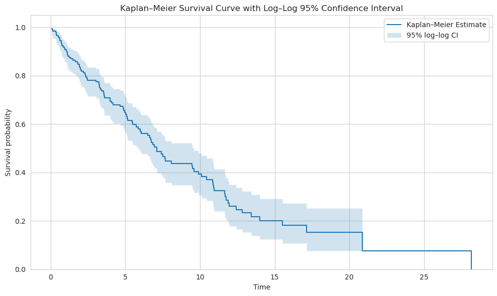
The output of the estimator is the KM curve, which is a step function where the drops occur at observed event times. It naturally incorporates censored data by adjusting the number of “at-risk” individuals at each step.

Kaplan-Meier Estimator is primarily used for descriptive analysis in scope of the survival analysis and comparing survival curves between two or more groups (e.g., treatment A vs. treatment B).

The Survival Function

The KM estimate is calculated as a product of conditional survival probabilities at each distinct event time.

\[\hat S(t) = \prod_{t_i \leq t} \left(1-\frac{d_i}{n_i}\right)\]

Where:

• $t_i$ is the time of the i-th distinct event.
• $d_i$ is the number of events (failures) observed at time $t_i$.
• $n_i$​ is the number of subjects at risk (alive and under observation) just before time $t_i$.

The resulting $\hat S(t)$ is a step function that only changes value at the points where an event occurs.

Confidence Interval Calculation

Before calculating the Confidence Interval we must have the variance at hand.

Calculation of the Variance

Taking logs turns the product into a sum; the variance of that sum is the sum of variances of the increments.

\[\ln \hat S(t) = \sum_{t_i \leq t} \ln \left(1- \hat p_i \right)\]

where $\hat p_i$ is ${d_i}/{n_i}$.

For each term $\ln(1-\hat p_i)$ we can approximate its variability using a Delta Method linearization:

\[Var [\ln(1-\hat p_i)] \approx \left[\frac{d}{dp}(1-p)|{}_{p=p_i} \right]^2 Var(\hat p_i) = \frac{1}{(1-p_i)^2}Var(\hat p_i)\]

$\hat p_i$ is a binomial proportion which is approximated via the normal distribution with variance $Var(\hat p_i)\approx p_i(1-p_i)/n_i$. Then,

\[Var [\ln(1-\hat p_i)] \approx \frac{1}{(1-p_i)^2} \cdot \frac{p_i(1-p_i)}{n_i} = \frac{p_i}{n_i (1-p_1)}\]

By replacing back $p_1$ with ${d_i}/{n_i}$ we get this:

\[Var [\ln(\hat S(t))] \approx \sum_{t_i \leq t} \frac{d_i}{n_i (n_i-d_1)}\]

Finally, use the delta method again to go from $\ln \hat S(t)$ to $\hat S(t)=\exp(\ln\hat S(t))$:

\[Var[\hat S(t)] \approx S(t)^2 Var [\ln(\hat S(t))]\]

The finally we obtain the Greenwood’s formula:

\[Var[\hat S(t)] = S(t)^2 \sum_{t_i \leq t} \frac{d_i}{n_i (n_i-d_1)}\]

Common Confidence Interval (CI) Constructions

There are multiple ways to calculate the CI.

1. Wald CI (simple, but can give limits outside $[0,1]$):

\[\hat S(t) \pm z_{1-\alpha/2}\sqrt{Var(\hat S(t))}\]

1. Logarithmic transform CI (stabilizes multiplicative variability):

Let $g(S)=\ln S$. Then $g’(S)=1/S$ and by the delta method:

\[Var(\ln \hat S(t)) \approx \frac{Var(\hat S(t))}{\hat S(t)^2} = \sum_{t_i \leq t} \frac{d_i}{n_i (n_i-d_1)}\]

Let’s mark this expression as $V(t)$, then a $(1-\alpha)$ CI for $\ln S$ is

\[\ln \hat S(t) \pm z_{1-\alpha/2}\sqrt{V(t)}\]

Back-transform (exponentiate) to get a CI for $S(t)$:

\[[\hat S(t)e^{-z\sqrt{V}}, \hat S(t)e^{+z\sqrt{V}}]\]

where $z = z_{1-\alpha/2}$

This keeps bounds positive and is multiplicative.

1. Log–log (or complementary log–log) transform CI (widely used; good small-sample coverage and stays in $[0,1]$):

Let $g(S)=\ln\big(-\ln S\big)$. Note $g$ is now defined for $0<S<1$. Then compute derivative:

\[g'(S) = \frac{d}{dS}\ln(-\ln S) = \frac{1}{S \ln S}\]

Apply the Delta Method:

\[Var(g(\hat S)) \approx [g'(S)]^2 Var(\hat S) = (\frac{1}{S \ln S})^2 S^2 V(t) = \frac{V(t)}{(\ln S)^2}\]

Replacing $S$ by $\hat S$ we get the estimated standard error.

\[SE[g(\hat S(t))] = \frac{\sqrt{V(t)}}{|\ln \hat S(t)|}\]

The absolute value of $\ln \hat S(t)$ is used to ensure that the standard error is positive. The confidence inteval on $g(S)$:

\[g(\hat S(t)) \pm z \cdot \frac{\sqrt{V(t)}}{|\ln \hat S(t)|}\]

Invert the transform to get a CI for $S(t)$. The inverse function is

\[S=\exp⁡(−\exp⁡(g))\]

Because $S = \exp(-\exp(g))$ is decreasing in $g$, when mapping the two end points you must swap them. The conventional formulas are:

\[\text{Lower CI} = \exp\left[-\exp\left(\ln(-\ln \hat S(t)) + z \cdot \frac{\sqrt{V(t)}}{|\ln \hat S(t)|}\right)\right]\] \[\text{Upper CI} = \exp\left[-\exp\left(\ln(-\ln \hat S(t)) - z \cdot \frac{\sqrt{V(t)}}{|\ln \hat S(t)|}\right)\right]\]

Practical Notes and Edge Cases

• If $\hat S(t)=0$ or $\hat S(t)=1$ exactly, the log or log–log transforms are undefined. In practice you avoid trying to transform at exact 0 or 1 (e.g. report one-sided CIs, or stop at the last time where $\hat S>0$, or use small continuity adjustments).
• The simple Wald CI can produce negative lower bounds or upper bounds >1 — this is why log or log–log transforms are preferred.
• The log–log CI works well especially for moderate sample sizes and when the survival is neither extremely close to 0 nor 1.

Testing for Equality of two Estimators: Log-Rank Test

The log-rank test is the natural nonparametric comparison test — it compares observed and expected events at each time using hypergeometric (or approximated binomial) allocation, and sums the standardized differences; it is asymptotically $\chi^2_1$ for two groups.

Compare survival experience of two groups (say group 1 and group 2). Null hypothesis:

\[H_0: \text{hazard functions are equal} (\lambda_1(t) = lambda_2(t) \forall t)\]

or equivalently the survival curves are the same.

At each time event $t_i$:

• $n_{1i}, n_{2i}$ be numbers at risk in group 1 and 2 just before $t_i$,
• $n_i = n_{1i}+n_{2i}$,
• $d_{1i}, d_{2i}$ be observed events at $t_i$ in the two groups,
• $d_i = d_{1i} + d_{2i}$.

Under $H_0$, given that $d_i$ events happen at time $t_i$ among the $n_i$ at risk, the number assigned to group 1 has a hypergeometric distribution (choose $d_i$ from $n_i$ without replacement). Thus the expected number of events in group 1 at time $t_i$ is:

\[E_{1i} = n_{1i}\frac{d_i}{n_i}\]

and the variance (hypergeometric variance) is:

\[Var(d_{1i}) = \frac{n_{1i} n_{2i}}{n_i^2} \cdot d_{i} \cdot \frac{n_i - d_i}{n_1 - 1}\]

Here is some intuition behind this formula:

• $\frac{n_{1i} n_{2i}}{n_i^2}$ is the relative mixing between groups (if one group is small, variance drops).
• $d_i$ is number of total failures — more failures → more randomness in who fails.
• $\frac{n_i - d_i}{n_1 - 1}$ is the finite-population correction: drawing without replacement reduces variability.

If $n_i$ is large, the factor $(n_i-d_i)/(n_i-1)$ is close to 1 and the variance approximates the binomial form.

The log-rank statistic

Form the sum of observed minus expected events over all distinct failure times:

\[U = \sum_{t_i} (d_{1i} - E_{1i})\]

Under $H_0$ the mean of $U$ is 0. The variance of $U$ is

\[Var(U) = \sum_{t_i} Var(d_{1i}) = \sum_{t_i} \frac{n_{1i} n_{2i} d_i (n_i - d_i)}{n_i^2(n_1 - 1)}\]

Then we can calculate z-statistic as

\[Z = \frac{U}{\sqrt{Var(U)}}\]

For large samples $Z\approx \mathcal {N}(0,1)$ under $H_0$, so the usual test uses

\[\chi^2 = Z^2 \approx \chi_1^2\]