Tree-like algorithms
The tree-like algorithms are a wondrous array of machine learning methods that draw inspiration from the branching structure of the natural world. They employ decision trees or ensemble techniques that combine multiple decision trees to make predictions, and are commonly used in classification and regression problems.
The decision tree algorithms, such as the classic decision tree and random forest, are much like the old oak trees of the forest. They have a trunk that represents the main decision path, and branches that represent the possible outcomes. These algorithms are often employed due to their ease of interpretation and their ability to handle both categorical and numerical data.
In this article
Decision tree
The decision tree is one of the building blocks in the realm of machine learning and data analysis. It is a type of algorithm that utilizes a branching structure to make decisions based on the values of input variables, and is commonly employed in supervised learning.
The process of constructing a decision tree involves recursively splitting the data into subsets, based on the values of the input variables. At each node of the tree, the most important feature is selected, and the data is split based upon its value. The criterion for splitting may be based upon entropy, information gain, or other measures of uncertainty or impurity reduction for classification problems, or upon the loss function such as mean squared error in case of regression problems.
To evaluate a split point, the algorithm computes the impurity or loss measure before and after the split for each candidate feature and split point. The reduction in impurity or loss is then calculated as the difference between the pre-split and post-split impurity or loss. The candidate split point that results in the largest reduction is selected as the best split for that feature.
It is worth to note that when evaluating the importance of the features, decision trees favor those with high cardinality because they contribute more to distinct data separation (no or little further splitting is required).
This process is repeated recursively for each child node until a stopping criterion is met, such as reaching a maximum depth or minimum number of samples per leaf node. The resulting tree consists of a series of nodes, where each node represents a feature and split point, and each leaf node represents a prediction value or class label.
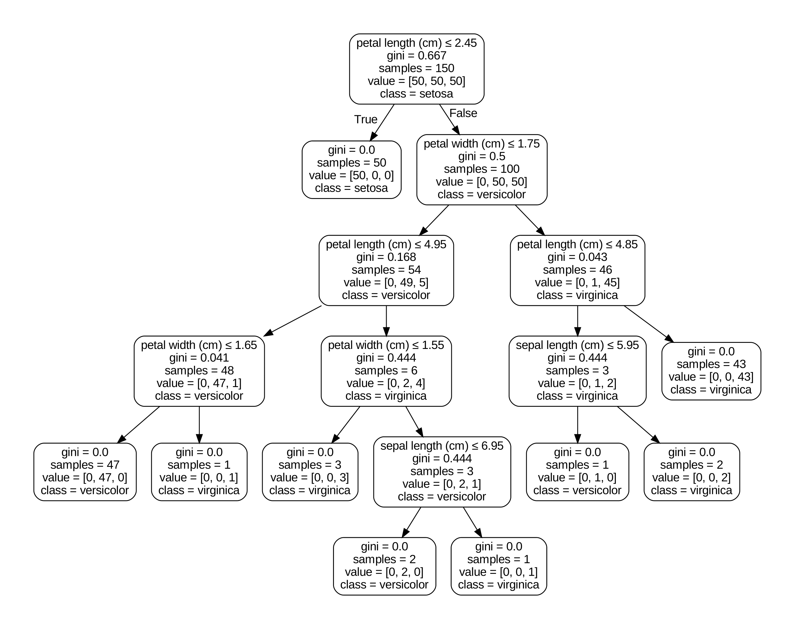
Once the tree is fully grown, it may be used to make predictions for new data points, by traversing the tree from the root to the appropriate leaf node. Each internal node in the tree represents a decision based on a feature’s value, and each leaf node represents a predicted class or outcome. Below is an example of a decision path of the algorithm when determining the type of an iris plant.
In case of a regression task the decision tree employs averaging at the leaf level so it is also capable of making continuous predictions.
The decision tree is a useful basic tool, as it can handle both categorical and numerical data, and is easily interpreted and visualized. However, it is susceptible to overfitting, and may require pruning or other measures to ensure its accuracy. Moreover, small changes in the data may result in different trees being constructed, and this should be kept in mind during usage.
Random forest and bagging
The random forest is an improvement over the decision tree algorithm where it assembles many trees at once, each using a random sample from the original dataset, and only a random subset of features. The results of individual decision trees are combined by averaging or voting, to improve the accuracy and robustness of the model.
The process of sampling subsets of the training data with replacement and training on each subset and then aggregating their predictions to obtain the final output is known as bootstrap aggregation or bagging.
Since each tree is constructed using a slightly different set of data and features, this helps to reduce the variance and overfitting of the individual trees. The shortcoming of the random forest however is that it can be computationally expensive to train and may require more hyperparameter tuning compared to a single decision tree such as the number of trees, the size of the data used for a single tree, and the number of features.
The importance of the features is determined by the mean decrease in impurity (MDI) which is the average version of the impurity decrease computed along all trees.
A faster version of the random forest is extremely randomized trees (or extra trees). It is different in a way that for each tree the threshold for splitting is not searched for in the space of the feature values but instead selected as the best one from the randomly drawn thresholds. Compared to the random forest, this approach may further reduce variance but the bias may be increased. Back to top ↑
AdaBoost
AdaBoost is an example of a model which utilizes the idea of boosting, namely combining weak learners into a strong one, and it does so by taking the weighted average from their predictions. Usually a small decision tree or a tree stump (one node and two leaves) is used as a week learner.
The learning in scope of the AdaBoost model is done iteratively. At first equal weights are assigned to the data points, and they are fed to a weak learner. Then the weights are adjusted so that those data points which were incorrectly predicted (or have the biggest error) get higher weight, and fed to a new weak learner. In this way the model gets focused on the data points that are difficult to predict, which can lead to better performance on the overall dataset. The individual learners themselves also get the weights which are based on their performance on the training set. Back to top ↑
Gradient boosting
Gradient tree boosting, also known as the Gradient boosting machine (GBM), is another example of boosting when weak learners are combined together to produce a strong model. Unlike in AdaBoost the learners are combined not as a weighted sum but instead are added sequentially. So for $M$ weak estimators the predicted values are adjusted like this:
\[F_m(x) = F_{m-1}(x) + h_m(x)\]where $h$ is an estimator.
The final prediction is equal to this:
\[\hat{y}_i = F_M(x_i) = \sum_{m=1}^{M} h_m(x_i)\]The estimators are usually decision trees, and at each iteration they are fitted in a way that corrects the previously made errors with respect to minimizing the total loss. With the exception of the first iteration the estimators predict the residuals rather than the actual values.
\[h_m = \arg\min_{h} L_m = \arg\min_{h} \sum_{i=1}^{n}l(y_i, F_{m-1}(x_i) + h(x_i))\]where $l$ is a loss function, $n$ is the number of samples.
The model utilizes the concept of the gradient descent by considering the slope of the loss function at the current point $F_{m-1}(x_i)$. This slope is the gradient in the space of the data points where each sample has its own value of the derivative) with respect to the predicted value:
\[g_i = \frac{\partial l(y_i, F_{m - 1}(x_i))}{\partial F_{m - 1}(x_i)}\]The minimization of the total loss is achieved by moving along the slope in the direction of the minimum, and the negative gradient sets this direction. Therefore, the negative gradient becomes the target prediction value for the estimator $h$.
Since the slope might change its direction at any time, the change to the previously made predictions is made in small steps using the learning rate as in the regular gradient descent. Eventually the update rule can be expressed like this:
\[F_m(x) = F_{m-1}(x) + \alpha h_m(x)\]where $\alpha$ is the learning rate. Back to top ↑
Histogram-based gradient boosting
An enhanced version of GBM, also known as LightGBM, was originally developed by Microsoft to be computationally efficient for large samples. Under the hood for each continuous input feature it performs grouping of the samples using histograms of integer-valued bins which reduces the number of splits to consider. This also has the benefit that the sorting of values within nodes is no longer required.
The key feature of LightGBM is its use of the Gradient-based One-Side Sampling (GOSS) algorithm and Exclusive Feature Bundling (EFB) technique, which can significantly speed up the training process and reduce memory usage.
Specifically, GOSS first calculates the gradients of the loss function with respect to each sample in the training data. It then sorts the samples based on the absolute value of their gradients, and divides them into two groups: a large group containing the samples with small gradients, and a small group containing the samples with large gradients. The small group of samples is then selected for use in the training process fully, while the large group is sampled. This approach allows GOSS to focus on the most informative samples in the training data.
EFB on the other hand works by grouping together similar features into bundles and treating them as a single entity, thereby reducing the number of splits needed in each tree. The similar features are identified based on their importance scores, which are calculated during a preprocessing step before the training process begins. The importance scores are based on the split gain of each feature, which represents the improvement in the objective function (e.g., mean squared error) achieved by splitting on that feature. LightGBM applies hierarchical clustering in order to group together features which will likely result into the same split.
In the case of categorical features, LightGBM first converts them into numerical features using an encoding method such as one-hot encoding or frequency encoding. It then applies EFB to the resulting numerical features.
Many operations under the algorithm can be performed in parallel which enables faster computation, for example building histograms over different features and finding the best split points over them, calculating the gradients for different samples, making predictions.
In addition, some implementations of the histogram-based gradient boosting have an in-built support for missing values as they are placed into a separate bin or category during the histogram construction process. During the training process, when a weak learner is fitted to the histogram, it can treat the missing value bin as a separate category and learn to make predictions accordingly. If the missing values are encountered only in the test set then they are mapped to the mode value from a child node.
The model can also support weights for the training samples, and during training the gradients are multiplied by the respective weights. Back to top ↑
Xgboost
Xgboost, short for Extreme gradient boosting, is yet another enhancement of the gradient boosting algorithm which similarly to LightGMB relies on the histogram binning and parallelisation. There are some considerable differences however.
- XGBoost uses regularization to prevent overfitting and improve the generalization of the model.
- The histogram-based splitting is done using the histogram statistics unlike the gradient-based approach which is used by LightGBM, which makes Xgboost less efficient.
- In addition, Xgboost requires one-hot encoding of the categorical features while LightGBM does so automatically and uses the benefits of EFB.
- LightGBM is generally faster and more scalable than XGBoost, especially for large datasets with many features. This is due to its use of gradient-based splitting, GOSS, and EFB, which can reduce the computational cost and memory usage of the algorithm.
- XGBoost abides with the level-wise splitting strategy. In this approach, the algorithm scans through all possible split points for each feature at each level of the tree, and selects the one that results in the greatest reduction in the objective function. In contrast, LightGBM uses a leaf-wise tree growth strategy, where it selects the leaf node that has the highest gain and splits it, which leads to faster convergence. In this approach, the algorithm does not scan through all possible split points for each feature at each level, but instead focuses on the most promising split points based on the gradients and histograms built during training.
- XGBoost may be more accurate than LightGBM in certain scenarios, especially when the dataset is small and the number of features is low. This is because XGBoost can handle feature interactions more effectively than LightGBM by using a combination of first-order and second-order gradients. The level-wise splitting has also a contribution to that because it avoids catching the effect of the outliers.
- XGBoost has more hyperparameters to tune than LightGBM, which can make it more difficult to find the optimal set of hyperparameters. However, if the hyperparameters are tuned correctly, XGBoost can achieve better performance than LightGBM.
- XGBoost may be more accurate than LightGBM for imbalanced datasets where the number of instances in the minority class is much smaller than the majority class. This is because XGBoost has built-in support for handling imbalanced datasets.