Non-linear regression

Although application of linear regression is straightforward and characterized by many useful statistical properties, in the real life many processes have non-linear behaviour, especially in a long run.

Linear regression is well-behaved since the change in independent variables results in proportional change in the dependent value - it’s basically just a linear combination of the predictors. In case of non-linear regression this is not true anymore since the same change in the predictors results in a different change of the dependent variable at different points. Consider the examples below:

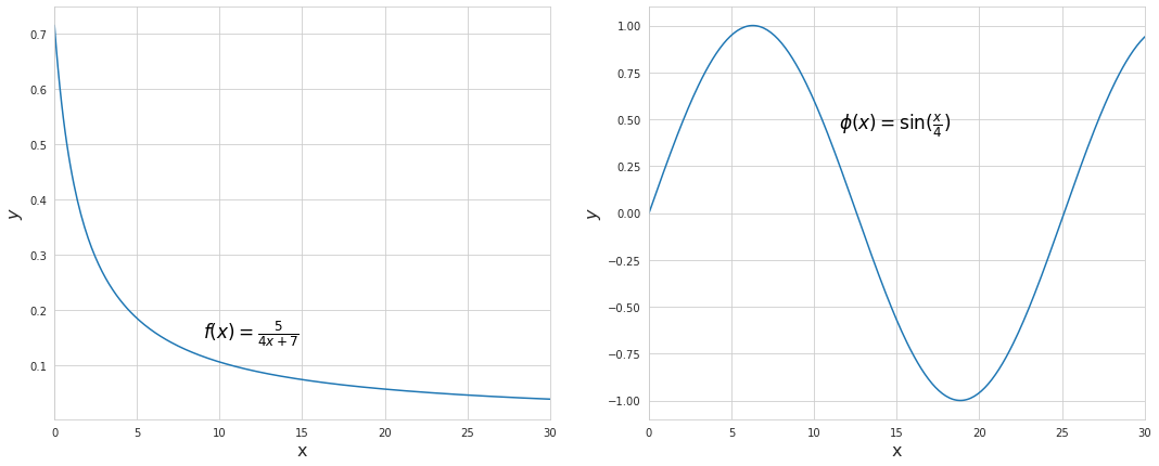
Both are just simple univariate functions, however they clearly demonstrate non-linear patterns of how they change. For instance, for $f(x)$ going from 0 to 5 results in a change of more than 0.5, yet another similar step from 5 to 10 results in a change of merely 0.08.

While the best set of parameters for the linear regression can be found analytically, in case of non-linear regression they are found iteratively by adjusting the initial guess with successive approximations, as in gradient descent and Newton’s method. Both of these methods are described in separate articles as they build the core of non-linear optimization. Other algorithms extend their capabilities by combining ideas and simplifying computations. Below are descriptions of some other notable non-linear optimization algorithms.

Gauss-Newton method

Gauss-Newton algorithm is one of the simplest methods for non-linear least squares solving. Other, more advanced algorithms are actually based on Gauss-Newton and extend its capabilities while also dealing with its shortcomings. Let’s take a look at what happens under the hood and how it is different from the original Newton’s method.

In the standard case of quadratic loss function we want to minimize the sum of squared distances between the modeled and the actual observations. Suppose we have a set of $m$ observations and a non-linear function $f(x, \theta)$ which we want to fit to the observations, where $\theta$ is a set of parameters. The sum of errors which we want to minimize will take the following form:

     $g(\theta) = \sum_{i=0}^m r^2 = \sum_{i=0}^m (y_i - f(x_i, \theta))^2$

where $y$ is a set of $m$ observations, and $r$ are residuals.

In an $n$-dimensional space $J(\theta)$ has its minimum value at a point where its gradient is zero. The gradient can be expressed as a system of $n$ equations, where $n$ is the number of dimensions.

\[\begin{cases} \frac{\partial g(\theta)}{\partial \theta_1} = 2\sum_{i=0}^m (y_i - f(x_i, \theta)) \frac{\partial f}{\partial \theta_1} = 0 \\ \frac{\partial g(\theta)}{\partial \theta_2} = 2\sum_{i=0}^m (y_i - f(x_i, \theta)) \frac{\partial f}{\partial \theta_2} = 0 \\ ............................. \\ \frac{\partial g(\theta)}{\partial \theta_n} = 2\sum_{i=0}^m (y_i - f(x_i, \theta)) \frac{\partial f}{\partial \theta_n} = 0 \end{cases} => J_r^{T} r = 0\]

$J_r$ is a matrix of first derivatives (Jacobian matrix) of the error term $r$.

In Gauss-Newton method the function $f(x_i, \theta)$ is approximated with the first-order Taylor series (second-order in case of the original Newton’s method and an initial guess of parameters:

     $f(x_i, \theta) \approx f(x_i, \theta^{(k)}) + \sum_{i=0}^m \frac{\partial f}{\partial \theta_i} (\theta_i - \theta_i^{(k)})$

From this we can express the residual as follows:

     $r_i = y_i - f(x_i, \theta) = y_i - f(x_i, \theta^{(k)}) - \sum_{i=0}^m \frac{\partial f}{\partial \theta_i} \Delta \theta_i^{(k)} = r_i^{(k)} - \sum_{i=0}^m \frac{\partial f}{\partial \theta_i} \Delta \theta_i^{(k)}$

where $r_i^{(k)}$ is the difference between the observed values and the values of a function with guessed parameters.

From here we get a system which will be possible to solve for $\Delta \theta$:

     $J_r^{T} r = 0$

     $J_r^{T}(r^{(k)} - J_r \Delta \theta) = 0$

     $J_r^{T} r^{(k)} = J_r^{T} J_r \Delta \theta$

     $\Delta \theta = (J_r^{T} J_r)^{-1} J_r^{T} r^{(k)}$

Eventually we get a vector of differences which should be applied to the parameters in order for them to ensure the minimum of the loss function for a given approximation. After that the procedure is repeated through repetitive approximation at a new set of parameters each time until the sum of squared errors becomes small enough or other stopping criterion reached.

Compared to the Newton’s method, Gauss-Newton is easier to implement and compute as it does not require calculation of the matrix of second derivatives and its inverse. If we compute the vectors of parameters change for Newton’s method we will get the same expression but with the Hessian instead of $J_r^{T} J_r$.

Here is what the Jacobian of the loss function looks like:

     $J_r = 2\sum_{i=0}^m r_i \frac{\partial r_i}{\partial \theta_j}$

According to the rules of differentiation, the Hessian can be expressed like this:

     $H = 2\sum_{i=0}^m (\frac{\partial r_i}{\partial \theta_j} \frac{\partial r_i}{\partial \theta_i} + r_i\frac{\partial^2 r_i}{\partial \theta_j \partial \theta_i}) = 2(J_r^{T} J_r + Q)$

where $Q = \sum_{i=0}^m r_i\frac{\partial^2 r_i}{\partial \theta_j \partial \theta_i}$

Gauss-Newton method may be seen as the result of neglecting with $Q$ in the Newton’s method. While it simplifies computations, convergence may be expected when either $r_i$ or $\frac{\partial^2 r_i}{\partial \theta_j \partial \theta_i}$ are small in magnitude (the function is “mildly” non-linear), as the method does not converge quadratically.

As long as $J_r$ has full rank, $J_r^{T} J_r$ always produces a positive definite matrix which is not guaranteed for the Hessian. Therefore, another advantage of Gauss-Newton method is that the descent direction is always towards the minimum. Still, the update vector may produce insufficient decrease of the objective function as it may cause overshooting of the minimum if the starting point is far from the true minimum. This can be fixed by taking a scaled version $\eta \Delta \theta$ on each iteration instead of $\Delta \theta$, where $\eta$ is between 0 and 1.The value of $\eta$ can be determined with line search methods such as backtracking line search. Another alternative is to use Levenberg–Marquardt algorithm.

Levenberg–Marquardt algorithm

The Levenberg–Marquardt algorithm, also known as the damped least-squares, employs a trust region approach in finding the minimum of a function, and can be seen as an improvement of the Gauss-Newton method. We have already described that Gauss-Newton method may be overshooting the minimum by making too big steps if the starting point is far from the minimum or if the function. Levenberg–Marquardt algorithm deals with the problem of slow convergence by interpolating between Gauss-Newton and gradient descent, shifting to gradient descent when the increase of the loss function is not sufficient. Therefore, compared to Gauss-Newton method, Levenberg–Marquardt is more robust as it can prevent overshooting the minimum, and navigates generally faster towards the minimum when the starting point is far off.

So Gauss-Newton method produces an update vector which is dependent of the Jacobian of the loss function:

     $\Delta \theta = (J_r^{T} J_r)^{-1} J_r^{T} r^{(k)}$

Levenberg–Marquardt algorithm modifies the square matrix $J_r^{T} J_r$ of this equation by adding to it multiple of the identity matrix $\lambda I$, where $\lambda$ is a positive number known as a damping factor. By increasing the diagonal elements $J_r^{T} J_r$ its eigenvalues are also increased. In addition, if the matrix is singular, it becomes invertable. Compared to Gauss-Newton the elements of the update vector $\Delta \theta$ in Levenberg–Marquardt algorithm become smaller because they are defined by the inverse of a matrix with bigger eigenvalues. Increasing the damping factor $\lambda$ causes the algorithm to behave more like gradient descent by taking small steps in the direction of the minimum.

     $\Delta \theta = (J_r^{T} J_r + \lambda I)^{-1} J_r^{T} r^{(k)}$

The value of $\lambda$ is reevaluated at each iteration: if the loss function is decreased then $\lambda$ is decreased for the next iteration, and the algorithm is allowed to make bigger steps - behave more like Gauss-Newton. Otherwise, if the step did not decrease the loss function, $\lambda$ is increased, and the algorithm is told to behave more like gradient descent.

It is recommended to adjust $\lambda$ according to the strategy of delayed gratification as it has a higher success rate and fewer Jacobian calculations when compared to the strategy of fixed adjustments or indirect search. According to this strategy, the damping factor is increased by a small fixed number and decreased by a bigger number after each successful step (the algorithm is “trusted” to make a bigger step). Although this slows the initial progress, the convergence will become faster near the point of the minimum.

A certain improvement to the algorithm would be to use instead of the identity matrix a diagonal matrix with the elements of $J_r^{T} J_r$. In this way the squared Jacobians on the diagonal of $J_r^{T} J_r$ are scaled appropriately to their own values, not just by the same fixed value. The inverse of this matrix will help to ensure that the movement is also performed along the directions of small gradients.

     $\Delta \theta = (J_r^{T} J_r + \lambda D^{T} D)^{-1} J_r^{T} r^{(k)}$

where $D$ is a diagonal matrix constructed with the diagonal elements of the Jacobian $J_r$.