LOESS

It is quite common to have a relation between two values represented as a scatterplot. However, visual representation of a scatterplot alone can often be non-informative if the data is sparse, noisy, and has outliers. We might want to estimate the possible relationship between variables by building a smooth line instead, so that we can learn more about the behavior of a process. We would also like to extrapolate the unknown values. LOESS is a non-parametric technique which does exactly that and provides an alternative to traditional regression models. LOESS (also referred to as LOWESS) stands for locally estimated (weighted) scatterplot smoothing, and its main purpose is describing local behaviour of some process without using any prior knowledge about the nature of this process. Unlike parametric regression models which rely on global relationship between variables, non-parametric models display more flexibility in representing the exact nature of observed events, taking into consideration local patterns. As such LOESS helps to pinpoint some of the relationships which would be overlooked by traditional parametric regression. Applying LOESS first during exploratory data analysis could also help in determining a non-linear model to be fitted later.

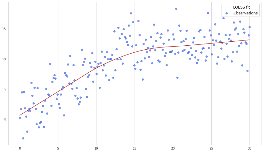
Below is an example of LOESS performed for some set of observations:

As we see, fitting linear regression in this particular case would not be wise as the process clearly changed its trend in the middle.

How it works

Smoothing with local regression

Given a set of $n$ observations we should select $m$ equally spaced points (they may not be represented by existing $n$ points). For each of these $m$ points the value is recalculated as a weighted average of a certain number of existing neighboring points where the nearest datapoints have the biggest weight.

Although we do not use parameters here for specifying the shape of the curve, a couple of hyperparameters should be specified beforehead in order to define the global behaviour of the algorithm. These are:

• the smoothing parameter $\alpha$ which determines the proportion of all observations used in a sliding window. Can have values between 0 and 1. Larger values of $\alpha$ produce smoother curves
• parameter $\lambda$ which determines the degree of the polynomial which is fitted to the points. $\lambda$ higher than 1 may help to capture the local curvature. The general rule is to set $\lambda$ to 1 when the function is expected to have monotonic behavious, and to 2 if the curvature of the line may produce local minima and maxima

The parameter $\alpha$ actually determines the number of points used in recalculation of each of $m$ points. One thing to note is that the number stays the same even if the point has neighboring values only to one side.

The weight of each of the nearest neighbours is determined by a tricube weight function:

     $w_i = (1-d_i^3)^3$

where $d_i$ is the fraction of the distance to $i$th point from the maximum distance. So if we are calculating the value of some $j$th point then $d_i$ the distance between this point and its $i$th neighbouring point divided by the distance between this point and the farthest point in its window.

All other points which are outside of the relevant window do not have any weight whatsoever.

Next, the parameters are estimated for each point of the local regression by minimizing the following expression:

     $\sum_{i=1}^{n}w_i(y_i - \sum_{k=0}^{\lambda}b_k x_i^k)^2$

This expression basically represents a weighted least squares cost function adjusted by the factor of $\lambda$ to allow polynomials in the main function.

Robustness step

Since local regression takes only a subset of observations the impact of outliers becomes more severe. Hence an additional robustness step may be performed within LOESS in order to remove the influence of outliers on the shape of a curve. Here is how it is done.

First of all the errors are calculated based on the results of the previous smoothing:

     $e_i = y_i - \sum_{k=0}^{\lambda}b_k x_i^k$

Then the following measure is calculated for each of the errors:

     $e_i^* = \frac{e_i}{6 Median\lvert e\rvert}$

And if $e_i^*$ is smaller than 1 then a bisquare weight function is calculated for the $i$th point:

     $r_i = (1-(e_i^*)^2)^2$

If $e_i^*$ is greater than zero, then error at $i$th point is considered too big so it’s disregarded completely by assigning it zero weight.

After that the parameters are estimated by minimizing the following form:

     $\sum_{i=1}^{n}r_i w_i(y_i - \sum_{k=0}^{\lambda}b_k x_i^k)^2$

It’s worth to mention that the robustness evaluation can be performed several times in order to improve the model. However usually several passes of this step suffice as the effect from any further repetition decreases quite rapidly and the parameters stop adjusting.