Linear regression

14 minute read

Regression analysis is used for estimating the relationship between variables, usually one dependent and one or several independent variables. Having a regression model at hand, we can predict some continuous value of the dependent variable based on the values of independent variables.

What is linear regression

Single variable linear regression explains the relationship between single input variable and the output:

$y = a + bx + \varepsilon$,

where $a$ and $b$ are parameters which explain the behaviour of the dependent variable according to the values of the independent one, and $\varepsilon$ is the residual.

The general form of linear regression however is the multivariable one where multiple predictors are taken into consideration:

$y = \beta_0 + \sum_{i=1}^n \beta_i x_i + \varepsilon$,

where $\beta_i$ are the weights of each independent variable.

A key feature of linear regression models is that it is assumed that a certain change in the variables causes proportional change in the output (which is not the case in non-linear models). The output is basically treated as a linear combination of predictors. In the real life scenarios this behaviour can only be observed for short periods of time as many natural and social processes tend to have non-linear rate of change. Back to top ↑

Gaussian noise

In practice there are always factors which are impossible to explain and predict and which may cause surprisingly different results from those that we expect. Therefore there is always going to be some difference between estimated (predicted) and actually observed values - the residuals, even for the variables which seem to be perfectly correlated.

It is common to view the relationship between two observed variables on a scatterplot. Seeing each individual observation helps to estimate the level of variation of the dependent variable, as well as to identify outliers. Below is an example of a nearly linear relationship between two variables which exhibits a certain amount of variation.

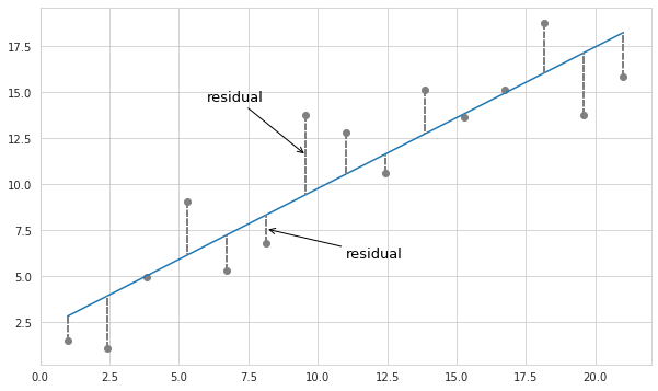
According to the Central Limit Theorem if the number of observations is large enough - the residuals have normal distribution with the mean value of 0. This basically means that for a modeled relationship between two or more variables the observed variation is mainly clustered around the estimated values. Since normal distribution is also called Gaussian distribution, the distribution of residuals around estimated values is called Gaussian noise. Back to top ↑

Matrix notation

For computation purposes it is better to represent the relationship between the dependent and independent variables with matrix notation:

$Y = X \beta + \varepsilon$,

where $Y$ is the group of all outputs and $X$ is the composition of all predictors for each particular output:

\[Y = \left[ \begin{array}{c} y_1 \\ y_2 \\ ... \\ y_n \end{array} \right] \text{ } X = \left[ \begin{array}{ccccc} 1 & x_11 & x_12 & ... & x_1n \\ 1 & x_21 & x_22 & ... & x_2n \\ ... & ... & ... & ... & ... \\ 1 & x_n1 & x_n2 & ... & x_nn \end{array} \right]\]

where $\beta$ is the vector of parameters (weights) of each predictor, and $\varepsilon$ is the vector of errors (Gaussian noise). This variable captures all other factors which influence the dependent variable y other than the regressors.

The parameters $\beta$ of such equation are usually estimated with least squares, however other methods such as maximum likelihood or robust estimation techniques can be employed. Back to top ↑

Confidence intervals of the coefficients

Recall that the confidence interval from a sample is the region around the sample mean, which with a certain probability contains the true mean.

$(\bar X - Z \cdot SE; \bar X + Z \cdot SE)$

where $Z$ is the critical value for a given significance level (confidence level minus 1), and $SE$ is the standard error.

In case of the linear regression the coefficients are calculated based on sample data so they should be viewed as sample means. The variances of the coefficients may be estimated with the covariance matrix, as described here. Then the standard error can be obtained by dividing them by the square root of the number of observations.

When we are dealing with a sample, and the true variance is unknown, instead of the critical value $Z$, which assumes the normal distribution, the $t$-value from the $t$-distribution is used. The number of degrees of freedom for the $t$-value in case of the linear regression is ($n$-$m$-1), where $n$ is the number of observations, and $m$ is the number of independent variables. Back to top ↑

Other assumptions

Apart from the linear nature of relationship between predictors and the output the linear regression estimation relies on a number of other assumptions:

Absence of perfect multicollinearity among predictors - that is that none of the predictors can be expressed as a copy or a linear combination of other predictors.
Independence of errors - absence of correlation among errors in different output values.
Normal distribution of the error term with the mean value of 0.
Homoscedasticity - constant variance of the error term regardless of the values of independent variables.

If not all of the assumptions are satisfied then the model might not have some of the required variables which explain the behaviour of errors, or instead might have redundant variables causing multicollinearity. Or maybe the relationship among variables is non-linear.

If the errors are correlated and/or heteroscedastic, instead of minimizing the sum of squares ($\varepsilon^{T} \varepsilon$), the following Mahalanobis distance has to be minimized: $\varepsilon^{T}\Omega^{-1}\varepsilon$. Where $\Omega$ is the covariance matrix of the errors, which is not equal to the identity matrix as in the case of homoscedastic independent errors.

Then in order to estimate the parameters, instead of the ordinary least squares (OLS) the generalized least squares provides the best estimation by taking into account the covariance of the error term:

$\beta = (X^{T}\Omega^{-1}X)^{-1}X^{T}\Omega^{-1}Y$

In practice however, the true covariance matrix is not known so it needs to be estimated from the sample. In this case the method of solving is called feasible generalized least squares (FGLS). Back to top ↑

Hypothesis testing in linear regression

In scope of linear regression we may want to test the significance of the model in general, and the significance of each individual parameter.

Significance of the parameters

When testing the parameters we perform the hypothesis test of whether a given parameter is equal to 0:

$H_0: \beta_i = 0$

$H_a: \beta_i \ne 0.6$

So for a given significance level the $t$-statistic is calculated:

$t = \frac{\beta_i - 0}{SE_i}$

where $SE_i$ is the standard error of the $i$th coefficient.

If the resulting $t$-statistic has corresponding $p$-value less than the significance level then the null hypothesis is rejected, and the parameter of the regression is considered significant. Back to top ↑

Significance of the model

In essence this test checks whether inclusion of independent variables (all at once) makes a better model than the model without independent variables.

The null hypothesis here implies that all of the coefficients at independent variables are equal to 0, and the alternative would mean that at least one of them is not equal to zero. The test statistic in this case would be F-test.

On the whole, there might be cases when the model in general is statistically significant but each individual coefficient is not. This happens when the predictor variables are highly correlated among themselves. Due to multicollinearity the coefficient values become unstable, and their confidence intervals inflated, so these intervals include 0. Back to top ↑

Validation of assumptions

Linear regression via ordinary least squares is safe to apply if all of the assumptions are satisfied. Using the Boston houses prices dataset let’s perform a typical check in order to ascertain whether it is reasonable to apply linear regression to predict prices.

Linear relationship

This can be validated by checking correlation coefficients between predictors and the dependent variable. Coefficients with absolute values closer 1 hint at linear relationship between variables. Below is the plot of the relationship between price and some of the predictors.

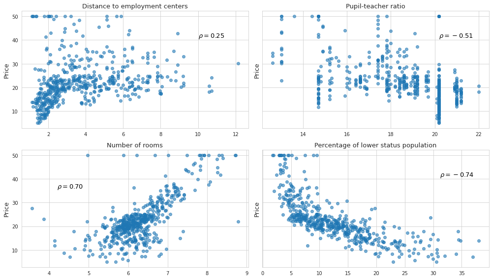
As we see, the percentage of lower status population, and number of rooms have higher coefficients of correlation, and seem to be raleted with the price. In addition, the percentage of lower status population exhibits non-linear trend. Pupil-teacher ratio shows weak correlation. And the distance to the employment centers at first doesn’t seem to matter at all, but we can clearly see some sort of linear but heteroscedastic pattern for smaller values of distance, and almost no pattern for higher values.

After visual inspection in becomes clear that one should not rely on the coefficients of correlation alone, since some of the variables might still be useful despite the low values of coefficients. Oftentimes it makes sanse to transform the predictors, for example by taking the logarithm, so that their values become monotonic and hopefully linearly related with the target variable. Back to top ↑

Absence of perfect multicollinearity among predictors

Similarly, in order to detect multicollinearity we may check correlation coefficients between predictors, as well as the pairplot of each combination of two variables.

From our example we see that the log transformed values of the criminal rate, the distance to the employment centers, as well as the value of nitric oxides concentration are related:

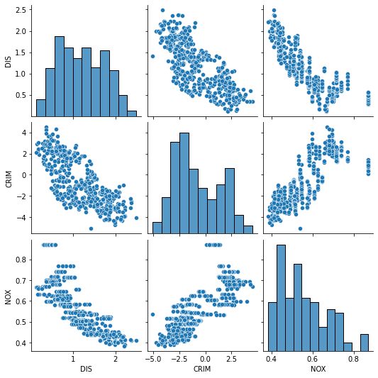
And yet, checking the pairwise distribution plots or the correlation coefficients alone is not enough since a particular variable may be dependent on multiple other variables. To tackle this problem we should check variance inflation inflation factor (more to in can be found here), as it measures the variance in coefficients caused by multicollinearity in the variables of the model.

For the variables which we eventually decided to keep in the model we get the following values of VIF:

Variable name	VIF
% of lower status population	2.49
Number of rooms	1.83
Distance to employment centers	1.76
Tax rate	1.71

Which overall looks accaptable.

Multicollinearity could also be detected when the sign coefficient at a certain parameter is not what we would expect. This happens if the model tries to compensate for the effect of several correlated predictors. Also, if the coefficients are estimated multiple times using different samples - as the consequence of the inflated variance the estimations of highly correlated variables will be unstable. This leads to the situations when the overall significance of the model is high while each individual predictor is not statistically significant.

High condition number of the covariance matrix of predictor variables means that there is at least one direction in which the variance is almost non-existent. This also indicates multicollinearity because the number of dimensions may be reduced without losing much of the variation. Some methods, such as singular value decomposition may be used to deal with multicollinearity internally by extracting new fully independent features, and selecting among them only those that capture the most of the variance in the dataset. Back to top ↑

Independence of errors

This assumption basically means that the residuals of the model do not form any pattern, and that there is no autocorrelation. Usually autocorrelation is present if the results of the previosu observation are impacting the future ones, but it may also mean that some of the important predictor variables are omitted from the model.

Below is the disribution of the residuals agains the predicted values of our model.

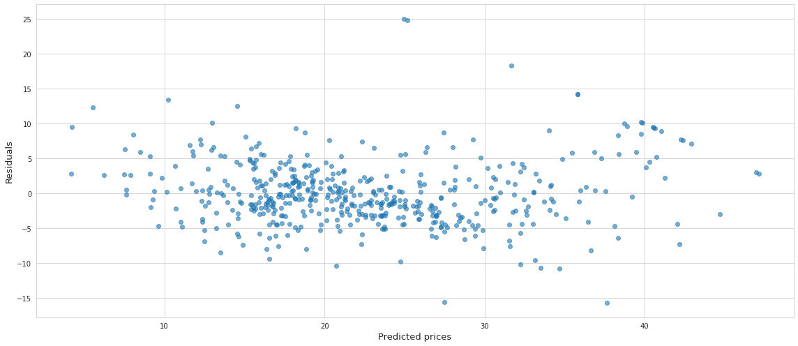
At first glance, there doesn’t seem to be any pattern, which is good.

If it is possible to determine the order of observations in the sample, then it is possible to test for serial correlation of the residuals using Durbin-Watson or Breusch–Godfrey test, which is no applicable in our case.

If however the tests were able to identify the autocorrelation of the errors then the obvious way to remove it is to add some of the omitted variables if they are known. However in practice this information is usually absent, so another way to deal with it is to add the lag of the dependent variable as an additional predictor. Let’s take a look at the Cochrane–Orcutt estimation which was designed specifically for this purpose. Suppose we have regression in form of

$y_t = \alpha + \beta X_t + \varepsilon_t$

And autocorrelation of the residuals at lag 1:

$\varepsilon_t = \rho \varepsilon_{t-1} + u_t$

where $u$ is the white noise, and $\rho$ is some coefficient which takes values from -1 and 1. By taking the difference (adjusted by $\rho$) between the residuals of consecutive results it is possible to replace the autocorrelated residuals with the white noise.

$\varepsilon_t - \rho \varepsilon_{t-1} = u_t$

$y_t - \alpha - \beta X_t - \rho(y_{t-1} - \alpha - \beta X_{t-1}) = u_t$

$y_t - \rho y_{t-1} = \alpha (1 - \rho) + \beta (X_t - \rho X_{t-1}) + u_t$

In order to find the coefficients of this final equation, first the values of $\alpha$ and $\beta$ from the base regression need to be estimated. Then $\rho$ is estimated from the residuals, and new values of the parameters are estimated from the equation built on differences adjusted by $\rho$. These new parameters are based on the assumption of autocorrelation of the residuals. Using them in the base equation a new value of $\rho$ is estimated, and the procedure is repeated until the convergence is reached.

A slightly better alternative would be Prais–Winsten estimation which is basically based on the Cochrane–Orcutt estimation but it doesn’t remove the first observation from the series when calculating lags. Intead, for $t$=1 it adds this expression:

$\sqrt{1-\rho^2} y_1 = \alpha \sqrt{1-\rho^2} + \beta \sqrt{1-\rho^2} X_1 + \sqrt{1-\rho^2} \varepsilon_1$ Back to top ↑

Normal distribution of errors

Estimation of the confidence intervals of the parameters of a model, as well as performing hypothesis tests on the parameters, relies on this assumption. Otherwise skewed distribution of the residuals would make these estimations and tests unreliable.

It is important to note that in the real life situations the perfect normal distribution is unachievable. This is primarily the reason why the formal tests of normality reject the hypothesis of the variable being normally distributed for big datasets.

In case of regression, usually if there is a linear relationship between the variables, and there is no autocorrelation of the residuals, the distribution of the residuals is close to normal.

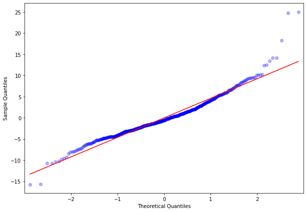
One way to visually inspect the degree of normality for the errors is to build a Quantile-Quantile (QQ) plot where the observed percentiles of the variable are plotted against theoretical ones. Below is the QQ plot of the residuals of our model which does not look perfect but also does not display strong departures from normality as well.

Heteroscedasticity of errors

Upon visual inspection of the residual plot we observe some degree of heteroscedasticity. Also both Breusch-Pagan and White test reject the hypothesis of homoscedasticity of errors in our model.

Despite the violation of homoscedasticity of errors, the estimates of the parameters obtained with the OLS remain unbiased, however their confidence intervals cannot be accurately determined. Recall that the variance of the regression coefficients can be calculated as $\sigma^2 (X^{T}X)^{-1}$, where $\sigma^2$ is the variance of the error term. Under the condition of heteroscedasticity this variance is no longer a fixed number.

If the errors are independent but heteroscedastic, then the covariance matrix of errors is diagonal with the elements equal to the different variance. By applying the idea of the generalized least squares, we can take the inverse of this matrix and use it for finding the new set of parameters for regression. The inverse of a diagonal matrix is yet another diagonal matrix which consists of the reciprocals of its elements. In case of the linear regression this inverse is known as the matrix of weights. So the weighted least squares (WLS) is meant to deal with heteroscedasticity of the residuals by assigning smaller weights to observations with larger variance. Essentially, applying WLS is the same as transforming the whole dataset by adjusting for the individual variance of errors of each observation, and then applying OLS to it.

In practice however, this true variance of the errors is unknown, so it has to be estimated from the sample after the initial OLS regression is built. Simply taking the squared values of each individual residual won’t do because we need to find the general relationship between the residuals and the independent variables. The recommended way to go is to build another regression where the logarithm of the squared residuals is modelled with independent variables.

$\log(\varepsilon^2) = X\beta^{*} + u$

where $u$ is some white noise, and $\beta^{*}$ is a new set of coefficients. The logarithm is used in order to make the relationship closer to linear, and also to dampen the effect of outliers.

From here the fitted values of $\varepsilon^2$ are recovered, and their reciprocals are used for the weight matrix of the WLS. It should be noted that since the weights are determined from merely an approximation of the error variance, the WLS may not remove heteroscedasticity completely. In practice if the heteroscedasticity is not evident by visual inspection, one may ignore it completely and just go with the OLS in order to safeguard himself from the possible false assumptions. Back to top ↑

Share on

Twitter Facebook LinkedIn