Linear mixed model
This type of model is suited when observations are not completely independent. Perhaps we measured the same individuals multiple times over a study, or we collected data from students nested within different schools. If so, we have likely encountered a common statistical challenge that traditional linear models (like simple linear regression) struggle with.
The problem is that standard linear models assume all observations are independent. When they’re not – when there’s a natural grouping or repeated measurements – these models can produce inaccurate results, including incorrect standard errors and misleading p-values. Trying to aggregate our data to satisfy independence also leads to a significant loss of valuable information. For example if we aggregate all datapoints coming from the same school into a single observation we may end up with too few data points.
This is where Linear Mixed Models (LMMs) come in. LMMs are a powerful and flexible extension of traditional linear models designed specifically to handle data that exhibits correlation or hierarchical/nested structures. They allow us to account for these dependencies, providing more accurate and robust insights into our data.
What are Linear Mixed Models?
At its core, a Linear Mixed Model (LMM) is a statistical model that incorporates both fixed effects and random effects to analyze data where observations are not independent.
Think of it this way: LMMs allow us to model variability at different levels of the data. We can model the average effect of certain factors (these are our fixed effects), while simultaneously acknowledging and accounting for individual or group-specific deviations from that average (these are our random effects).
Imagine we are studying the effectiveness of different teaching methods on student test scores. A fixed effect might be the specific teaching method itself – we want to know the average impact of “Method A” versus “Method B.” However, students are nested within different schools, and some schools might inherently perform better or worse due to factors not explicitly measured (e.g., school culture, resources). We are not necessarily interested in estimating the exact “effect” of each individual school, but rather in acknowledging that there’s school-to-school variability that needs to be accounted for. This school-level variability is captured by LMM by introducing the random effect into the equation.
Fixed Effects vs Random Effects: The Crucial Distinction
Understanding the difference between fixed and random effects is fundamental to grasping LMMs.
Fixed Effects
Fixed effects are those effects that are considered constant across the entire population or across all units being studied. We are directly interested in estimating the specific value of these effects.
They typically represent the primary independent variables (predictors) whose influence we want to quantify directly.
Examples: Specific treatment groups (e.g., “Drug A,” “Placebo”), gender (e.g., “Male,” “Female”), specific age categories (e.g., “Under 30,” “30-50,” “Over 50”).
Random Effects
Random effects are used to model the correlation structure in the data, often due to natural groupings or repeated observations on the same units.
Instead of being interested in the specific effect impact, we are interested in the variance component associated with these effects (e.g., “How much variability in outcome is explained by differences between schools?”), not necessarily the individual student’s specific deviation.
When to Use Linear Mixed Models? (Applications and Scenarios)
LMMs are incredibly versatile and are the go-to choice for a wide array of research designs where independence of observations cannot be assumed.
Hierarchical/Nested Data:
This is common when data naturally exists in layers. For instance, students are nested within classrooms, which are nested within schools. Patients might be nested within different hospitals, or employees within departments.
Example: If we are studying the impact of a new curriculum (a fixed effect) on student test scores, we’d use a random effect for ‘School ID’ to account for unmeasured differences between schools that might influence student performance, beyond the curriculum itself.
Repeated Measures/Longitudinal Data:
When we collect multiple measurements on the same individuals or units over time. These repeated measurements are inherently correlated because they come from the same source.
Example: Tracking the blood pressure of a group of patients over several weeks after they start a new medication. Each patient’s blood pressure readings over time are not independent; LMMs can model the trajectory for each patient while also identifying an average trend.
The LMM Equation
\[Y=X \beta+Zu+\epsilon\]Let’s break down what each part represents:
-
$Y$ is the vector of our observed outcome data – what we’re trying to predict or explain (e.g., student test scores, blood pressure readings).
-
$X$ is the design matrix for our fixed effects. It contains the values of our independent variables for which we want to estimate specific coefficients (e.g., indicator variables for treatment groups, age).
-
$\beta$ is the vector of fixed-effects coefficients. These are the parameters we estimate, telling us the specific impact of the fixed predictors on the outcome.
-
$Z$ is the design matrix for our random effects. It links our observations to their respective groups or units that introduce correlation (e.g., indicators for patient ID, school ID). The columns of the $Z$ matrix correspond to the random effects in our model, and its rows correspond to our observations. Each row will have a “1” in the column that matches the random effect for that observation and “0”s elsewhere.
-
$u$ is the vector of random-effects coefficients. Unlike $\beta$, these are not estimated as specific values but are assumed to be drawn from a statistical distribution (typically a normal distribution with a mean of zero). They represent the random deviations or adjustments for each group.
-
$\epsilon$ is the vector of residuals or errors. It represents the unexplained variation in our outcome variable, similar to the error term in traditional regression.
In essence, the equation states that the observed outcome is a combination of the average effects of the predictors (fixed effects), plus the unique adjustments for different groups or individuals (random effects), plus any remaining unexplained variability.
Challenges and Considerations
While powerful, Linear Mixed Models do come with their own set of considerations:
-
Computational Intensity: For very large datasets or models with highly complex random effects structures, LMMs can be computationally demanding, requiring more processing power and time.
-
Model Specification: Deciding which effects should be fixed and which should be random, and determining the appropriate correlation structure for the random effects, is often the most challenging aspect. This requires a good understanding of your research question and the underlying data structure.
-
Assumptions: While more flexible than traditional models, LMMs still rely on certain statistical assumptions, such as the normality of residuals and random effects, and homoscedasticity (constant variance) of residuals. Violations of these assumptions can affect the validity of your results, although LMMs are often more robust to minor deviations.
Example study: The Plant Growth Experiment
Imagine we are testing the effectiveness of two new fertilizers (“Fertilizer A” and “Fertilizer B”) compared to a standard “Control” group. We apply these treatments to ten different plots of land and measure the plants’ growth over five weeks.
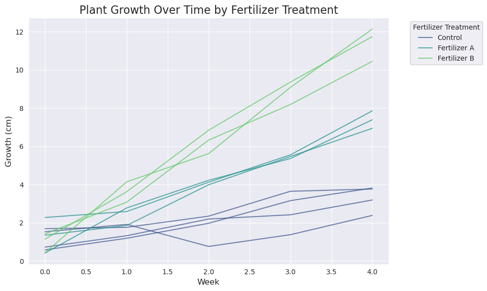
As we can see in the visualization, each colored line represents the growth trajectory of a single plant plot. The lines for each color are not perfectly parallel; this shows the natural variability between plots (the random effect). However, the lines for Fertilizer B generally have a steeper slope than those for Fertilizer A, which are in turn steeper than the Control lines. This demonstrates the overall, average effect of the fertilizer treatments, which is the fixed effect.
Why linear regression is not appropriate
If we were to use a simple linear model, we would treat each week’s measurement as an independent observation. However, the measurements from a single plot are not independent; the growth of a plant in one week is highly related to its growth in the previous week. Furthermore, the plots themselves are not identical—some might have naturally richer soil or receive more sunlight, leading to consistently faster growth regardless of the treatment.
How a Linear Mixed Model Solves This
A Linear Mixed Model addresses these issues by defining:
-
Fixed Effect: The Fertilizer Treatment (Control, Fertilizer A, Fertilizer B). You are specifically interested in estimating the average effect of each of these treatments on plant growth. This is the main question of your experiment.
-
Random Effect: The Plot ID. You don’t care about the specific growth rate of Plot 1 versus Plot 2; instead, you want to account for the inherent, unmeasured differences between the plots. The LMM models this variability as a random deviation from the overall average growth rate.
The equation for the plant growth experiment, using the notation from the LMM section, would look like this:
\[\text{Growth}_{ij}=\beta_{0}+\beta_{1}(\text{Week}_{ij})+\beta_{2}(\text{Fertilizer}_{A})+\beta_{3}(\text{Fertilizer}_{B})+u_{i}+\epsilon_{ij}\]Here:
- $\beta_{0}$ is the fixed intercept, representing the average baseline growth (at week 0) for the Control group.
- $\beta_{1}$ is the fixed slope, representing the average weekly growth rate for the Control group.
- $\beta_{2}$ is the fixed effect of Fertilizer A, representing how much its weekly growth rate differs from the Control group.
- $\beta_{3}$ is the fixed effect of Fertilizer B, representing how much its weekly growth rate differs from the Control group.
- $u_i$ is the random effect for plot $i$, representing the unique, plot-specific deviation from the overall average growth trajectory. This term accounts for the inherent differences between plots (e.g., soil quality). This is assumed to be a random variable, typically following a normal distribution $u_i∼N(0,\sigma_u^2)$.
- $\epsilon_{ij}$ is the residual error for plot $i$ at week $j$, representing the random, unexplained variation for that specific measurement. This is also assumed to be a random variable, typically following a normal distribution $\epsilon_{ij}∼N(0,\sigma_{\epsilon}^2)$.