Interpolation
Generally speaking, interpolation is a way of generating new data points which exactly fit into some given set of points. It is used for approximation of complex functions with simple ones, for example when estimating missing values among known data points.
Linear interpolation
Linear interpolation is rightfully one of the simplest types of interpolations. In it the unknown value is estimated by putting a straight line between two neighbouring datapoints with known values and setting an assumption that any missing value in between belongs to this line.
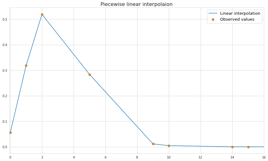
As we see, linear interpolation does a horrible job predicting the unknown values if the nature of the underlying process is non-linear.
Basically the slope between two datapoints is considered to be a slope of a function between these datapoints:
$\frac{y-y_a}{x-x_a}=\frac{y_b-y_a}{x_b-x_a}$
Piecewise constant interpolation
This technique is also known as nearest neighbour interpolation, and it consists of assigning the values of the nearest datapoints to the missing ones. Due to its simplicity this could be an option for multivariate cases.
Polynomial interpolation
Polynomial interpolation is perhaps the most well-known interpolation method which is used for finding a function which exactly fits a line into each of the given data points. For $n$ data points there always exists such function of at least $n-1$ degree. Also polynomial functions are smooth and continuous which allows calculation of $n-1$-degree derivative at any point.
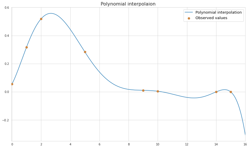
Although with polynomial function we can fit a line to any number of points, the error of a function will be increasing with the number of degrees of polynomial. Polynomial functions oscillate and the magnitude of oscillation increases for higher degree polynomials, which results into unnatural forms of a function at places other than the points to which the function was originally fitted. At the plot above we see how the function rapidly goes downward outside of the range of known datapoints. Just by eyeballing the known points of the function we may guess that it represents some sort of Poisson distribution. As we see, polynomial distribution does a good job approximating the missing values of a function but it is important to understand that if it’s a Poisson distribution indeed then its values cannot be lower than zero.
Below are some of the most used methods of calculating the polynomial function that interpolates know datapoints.
Vandermonde matrix
The most straightforward way to obtain polynomial function from $n$ given data point is to solve a system of $n$ linear equations where the parameters of the polynomial function are considered as variables. So for a function like this:
$p(x) = a_0 + a_1 x + a_2 x^2 + … a_n x^n$
we would have to solve the system by plugging all known values of $x$ and $y$:
\[\begin{cases} a_0 + a_1 x_1 + a_2 x_1^2 + ... a_n x_1^n = y_1 \\ a_0 + a_1 x_2 + a_2 x_2^2 + ... a_n x_2^n = y_1 \\ ............................. \\ a_0 + a_1 x_n + a_2 x_n^2+ ... a_n x_n^n = y_n \end{cases} => Xa = y\]Matrix $X$ used in this context is known as Vandermonde matrix. In practice this matrix is often ill-conditioned which causes errors in rounding of small floating point numbers.
Lagrange multipliers
The idea behind this method consists of forcing the polynomial function output to be equal to the actually observed value. This is achieved by representing the polynomial function as a sum of some basis functions.
$L(x_i) = y_i = \Sigma_{j=1}^{n}y_j l_j(x_i)$
This is the case when the following conditions hold true:
- $y_j l_j(x_i) = y_i$ while $i=j$
- $y_j l_j(x_i) = 0$ while $i \neq j$
Here the sum of functions becomes transformed into the sum of one number (which is equal to the actual function’s output) and zeroes. This in turn is achieved if:
- $l_j(x_i) = 1$ when $i=j$
- $l_j(x_i) = 0$ when $i \neq j$
It turns out that in order for $l_j(x_i)$ to satisfy all of the conditions from above it should have the following form:
$l_j(x_i) = \prod_{k=1}^{n}\frac{x_i-x_k}{x_j-x_k}$
where $k=j$ is skipped in order to avoid division by 0.
If $k=i$ then the numerator of one of the multipliers becomes 0 which in turn makes the whole expression equal to 0. Also if $i=j$ then numerators and denominators of each multiplier will cancel each other making the expression equal to 1.
Eventually interpolation with Lagrange multipliers is performed using this formula:
$L(x) = \Sigma_{i=1}^{n}(\prod_{k=1}^{n}\frac{x-x_k}{x_i-x_k})y_i$
Newton’s divided differences
The idea of this method is in gradual adjustment of polynomial function to account for each known datapoint in such a way that the progress made during fitting of previous points is not lost.
So this is how it works, for a first datapoint we have $f(x_1) = y_1$. In order to fit a function to just one line it is enough to set it as a constant line $f(x) = y_1$. Then we get the second datapoint $f(x_1) = y_1$ and adjust the function to pass through that point as well. This is achieved with the following expansion:
$f(x) = y_1 + \frac{y_2 - y_1}{x_2 - x_1}(x - x_1)$
So here $\frac{y_2 - y_1}{x_2 - x_1}$ is the expression of the slope between the two known datapoints, and $(x - x_1)$ is added in order to make the second term zero when $x = x_1$ so that the condition to pass through the first point is retained.
After that the third point is added, and the function is transformed again by taking the whole expression from the previous step and adding a new component which ensures satisfaction of the previous conditions.
$f(x) = a_1 + a_2{x_2 - x_1}(x - x_1) + a_3(x-x_1)(x-x_2)$
Here for simplicity of the formula we introduce coefficients $a$, where $a_1$ is the first coefficient $y_1$, $a_2$ is the first order difference $\frac{y_2 - y_1}{x_2 - x_1}$ and $a_3$ is a new coefficient whose meaning will be explained in a while. For now the important part is $(x-x1)(x-x_2)$ which ensures cancellation of the third term if $x = x_1$ or $x = x_2$ so that the progress made at previous steps remains intact.
During the previous step we added the factor of the first-order difference $a_2$ which became necessary for capturing the relation between change in values of two datapoints. After inclusion of the third point it became necessary to account also for acceleration of change (or in other words the change of change) between two spans: $x_1 - x_2$ and $x_2 - x_3$. Therefore, $a_3$ coefficient should capture the second-order difference between datapoints.
The process goes on like this after addition of each new datapoint and the general formula for the polynomial function looks like this:
$p(x) = a_1 + a_2(x-x_1) + a_3(x-x_1)(x-x_2) + … + a_n(x-x_1)(x-x_2)…(x-x_{n-1})$
Spline
Spline is a piecewise function which selects every two neighbouring datapoint and uses low-degree polynomials to interpolate between them. Splines is by far a better alternative to polynomial interpolation as they are less computationally expensive and tend to produce more realistic shapes of a curve, avoiding rapid oscillations. Below is the example of cubic spline (using third-order polynomials) interpolation for the same datapoints which were used for the linear and polynomial interpolation above.
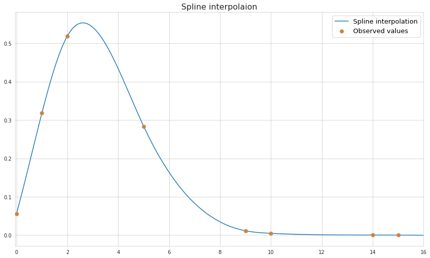
As we see, the shape of the function looks more realistic.
The idea behind constructing a spline is in finding $(n-1)$ polynomials for $n$ datapoints which satisfy certain conditions. First of all the values of the neighboring polynomials at the point where they join are equal - this ensures continuity. Also the function should pass through each of the known datapoints.
$p_i(x_i) = p_{i-1}(x_{i}) = y_i$
where $p_i(x_i)$ is a polynomial between points $x_i$ and $x_{i+1}$.
In order to ensure the smoothness of the function the first derivative at the meeting point of two polynomials should also be the same.
$p_i’ (x_i) = p_{i-1}’ (x_{i})$
Finally, forcing the second derivatives to be equal at the meeting point ensures the same rate of change at those points and the same shape of the curve.
$p_i’’ (x_i) = p_{i-1}’’ (x_{i})$
Cubic spline, that is a function consisting of third degree polynomials, is generally sufficient for meeting all of the conditions described above, hence this is a type of spline which is used the most.
In case of cubic spline we have 4 coefficients for each of the polynomials. Since there are $n-1$ polynomials for $n$ datapoints we have $4 \cdot (n-1)$ parameters for the whole system of equations.
Each of the points, except the first and the last one, are used in fitting both polynomials (before and after the point), giving $2(n+1)$ equations, while the first and the last one are used only once, giving 2 more equations. In addition, each of the inner points are used in equations of the first and the second derivatives. Bringing it all together we have $4n - 6$ equations. Combining this with the number of parameters we would get an underdetermined system of equations, so additional 2 constraints should be added.
One type of additional boundary condition is to force the first derivatives of the polynomials at $x_1$ and $x_n$ to be equal to some known values. This type of constraint is known as clamped boundary condition, and it roughly sets directions in which the function moves outside of the known datapoints. Another type of boundary condition is called natural or free, and it forces the second derivatives at $x_1$ and $x_n$ to be equal to zero. This in turn lets the function have the same rate of change at its first and last known datapoint, meaning that the direction of it won’t be changing.
Bezier curves
A Bezier curve is a mathematically defined curve which connects two points. It relies on the Bernstein polynomial which makes use of the control points. It could be viewed as a special case of spline interpolation which drops some of the requirements, in particular it does not care about the behavior of the curve beyond the two boundary points.
Bezier curves are widely used in computer graphics, computer-aided design (CAD), and other fields to represent smooth curves and shapes which can scale indefinitely.
Below are the equations for the main types of Bézier curves.
Linear Bezier curve, which connects two control points with a straight line:
\[B(t)= P_0 + t(P_1 - P_0) = (1−t)P_0+tP_{1}\]where $P_0$ and $P_1$ are the coordinates of the two points. $P_1 - P_0$ can be viewed as a displacement vector, and $t$ as its magnitude.
Quadratic Bezier curve, which connects two control points using the coordinates of third auxiliary point in order to make a curve as opposed to the straight line:
\[B(t)=(1−t)^2 P_0+2(1−t)tP_1+t^2 P_2\]It could be rewritten in a way which highlight the symmetry with respect to $P_1$, and which makes use of the the vectors pointing to this intermediary point:
\[B(t) = P_1 + (1-t)^2 (P_0 - P_1) + t^2 (P_2 - P_1)\]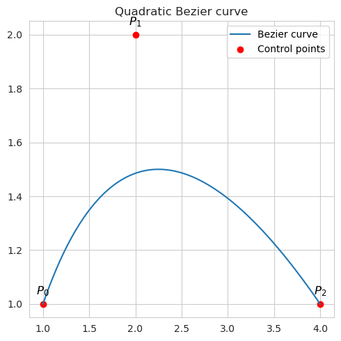
Cubic Bezier curve which is defined by four control points, allowing for more complex shapes: \(B(t)=(1−t)^3 P_0+3(1−t)^2 t P_1+3(1−t)t^2 P_2+t^3 P_3\)
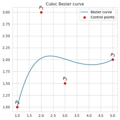
The control points serve as attractors, shaping the direction and curvature of the curve. The parameter $t$ can range from 0 to 1. The initial and concluding control points of the curve consistently represent the endpoints, with the intermediary control points generally not positioned directly on the curve. The curve’s position at any specific $t$ value is influenced by the weighted contributions of the control points.