Heteroscedasticity

What is heteroscedasticity

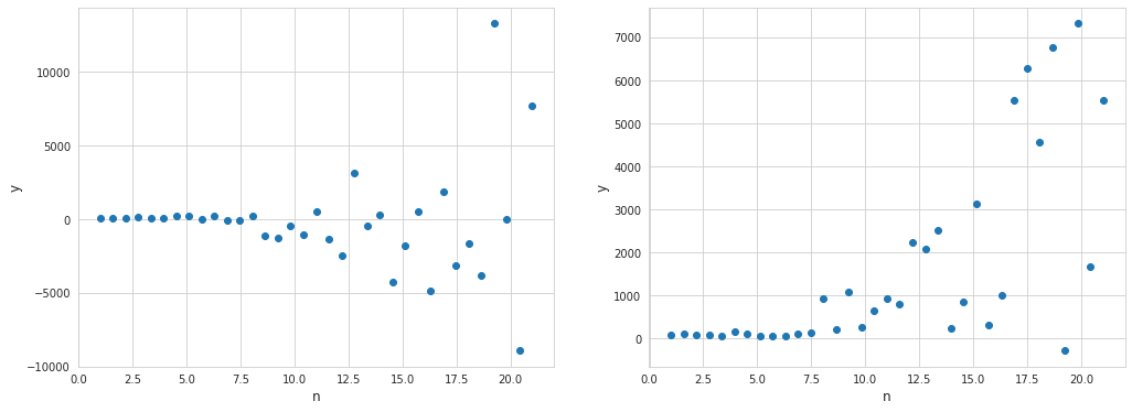
Heteroscedasticity is a situation when variability of a variable is unequal across the range of values of a second variable that predicts it. This actually means that the error is a function of an independent variable. Below are several examples of linear regression where heteroscedasticity came into play.

Among examples where heteroscedasticity may arise are relationships between:

• age and the average weight of a person
• years of work experience and salary
• company size and its net revenue

In regression analysis heteroscedasticity of residuals is something that would indicate the potential issues with the model. Although the estimates of the parametres with the ordinary least squares will be unbiased, the estimation of their variance will be unreliable.

On the contrary, homoscedasticity means constant variance of errors of a regression, regardless of the values of independent variables.

     $Var(\varepsilon_i \mid X) = \sigma^2$

And the covariance matrix of the residuals will be just $\sigma^2 I$. If however the variance of the errors is not constant, then the covariance matrix will be different:

\[Var(\varepsilon \mid X) = E(\varepsilon \varepsilon^{T}) = \Omega = \left[\begin{array}{cccc} \sigma_1^2 & 0 & ... & 0 \\ 0 & \sigma_2^2 & ... & 0 \\ ... & ... & ... & ... \\ 0 & 0 & ... & \sigma_n^2 \end{array} \right]\]

Testing for heteroscedasticity

Breusch–Pagan test

This test is meant to determine whether the variance of residuals in the regression model depends on independent variables. So at first the linear regression is built:

     $\hat y = \beta_0 + \beta_1 x_1 + \beta_2 x_2 + … + \beta_m x_m + \varepsilon_i$

The squared residual is then regressed against independent variables like this:

     $\varepsilon^2 = \gamma_0 + \gamma_1 x_1 + \gamma_2 x_2 + … + \gamma_m x_m + u$

where $u$ is the white noise. The null hypothesis states that all parameters $\gamma$ are equal to 0 - this will mean that there is no heteroscedasticity of the residuals as they won’t be dependent on any of the independent variables.

It turns out that the coefficient of determination of this new regresion multiplied by the sample size ($R^2 n$) under the null hypothesis is asymptotically chi-square distributed with $m$ degrees of freedom. The null hypothesis is rejected if the statistic is greater than the critical value of chi-square distribution for a given significance level.

R-squared indicates the goodness of the fit, so intuitively if its value is high - then the resulting statistic will be higher, hence the reason to reject the hypothesis of independence of the residuals from the predictors.

It is worth mentioning that this test assumes a linear relationship between the residuals and independent variables, so it may fail to identify heteroscedasticity in case of non-linear relationship.

White test

Unlike the Breusch–Pagan test this one one is meant to identify heteroscedasticity caused by non-linear relationships between predictors and residuals in the regression model. In addition to the linear form of regression, the squared residuals are fitted with the squared terms of independent variables, as well as their inner products:

     $\varepsilon^2 = \gamma_0 + \gamma_1 x_1 + … + \gamma_m x_m + \delta_1 x_1^2 + … + \delta_m x_m^2 + \eta_1 x_1 x_2 + \eta2 x_1 x_ 3 + … + u$

Having so many predictors will cause the significant loss of degrees of freedom, so another way to transform it, is to make use of the original estimate of $y$, so it becomes just this:

     $\varepsilon^2 = \gamma_0 + \gamma_1 \hat y + \gamma_2 {\hat y}^2$

Now this regression has ($n$-2) degrees of freedom, which eventually makes the test statistic more reliable. While the estimate of $y$ is a linear combination of independent variables, its square is a linear combination of squared independent variables and their inner products.

From here, the null hypothesis is that both $\gamma_1$ and $\gamma_2$ are equal to zero, meaning that the variance of residuals of the model does not depend on independent variables. Just like with the Breusch–Pagan test, the coefficient of determination of this new regresion multiplied by the sample size ($R^2 n$) under the null hypothesis is asymptotically chi-square distributed with 2 degrees of freedom.

A drawback of this test is that it can rapidly lose power if there are many independent variables.