Gaussian process
The Gaussian process may be viewed as a prediction technique which mainly solves regression problems by fitting a line to some given data (although it may be extended for classification and clustering problems as well).
In the essence the Gaussian process takes an infinite number of all possible regression estimations, and using the normal distribution it assigns probability to each of them. Then, the mean value and the standard deviation in the space of those estimations can be used for making predictions and building the confidence intervals.
In this article
- Preliminaries
- Realization of the Gaussian process
- Prior and posterior distribution in the Gaussian process
- Optimizing parameters
- Gaussian process at large datasets
Preliminaries
Multivariate Gaussian distribution
The Gaussian distribution is a core element upon which the whole idea of the Gaussian process is built.
Let’s take a look at two-dimensional examples of the Gaussian distribution with the mean at the origin and variance of 1 along each of the dimensions:
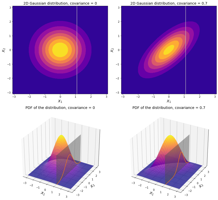
On the left-hand side the covariance is 0, which means that both dimensions are independent. So for example if an observation is spotted with a value greater than the mean along $X_1$ (like $X_1$ = 1.1 on the plot above) it has equal chances of being higher or lower than the mean along $X_2$.
On the contrary, if there is some non-zero covariance between two dimensions, then the distribution is no longer centered around the origin. As we see on the right-hand side of the charts above, the covariance is a positive number. So at $X_1$ = 1.1, which is greater than the mean along $X_1$, it is more likely that its value along $X_2$ is also greater than its corresponding mean.
All things considered, it makes sense to operate in terms of conditional probability, where the expected value of one variable (in our case $X_2$) depends on the observed value of another ($X_1$ in our example). Here is a neat mathematical property: if one normally distributed variable is conditioned on another normally distributed variable, then the resulting conditional distribution is also normal. In the visualization above we can see a familiar bell-shaped curve where a plane ($X_1$ = 1.1) slices through a bivariate normal distribution. This curve exactly defines the probability density function of the conditional distribution here. Back to top ↑
Conditional distribution properties
Suppose there is a set of variables which is split into two parts: $X$ and $Y$. Either of them may be a single dimension or a vector containing multiple dimensions. Assuming that both $X$ and $Y$ are normally distributed, it is possible to calculate the conditional mean and the conditional covariance matrix. As stated above, the resulting conditional distribution will be also Gaussian.
\[\left(\begin{array}{c}X\\ Y \end{array}\right) \sim \mathcal{N} \left(\left(\begin{array}{c}\mu_X\\ \mu_Y \end{array}\right), \left(\begin{array}{cc} \Sigma_{XX} & \Sigma_{XY} \\ \Sigma_{YX} & \Sigma_{YY} \end{array}\right)\right)\]Here $\mu_x$, $\mu_y$ are respective means of $X$ and $Y$, which are either numbers or vectors depending on whether $X$ and $Y$ contain more than one variable.
If $X$ is a single vector then $\Sigma_{XX}$ is just a number which corresponds to the variance within the variable. If however $X$ contains more than one variable then $\Sigma_{XX}$ is the variance-covariance matrix of the variables within $X$. Same goes for $\Sigma_{YY}$.
$\Sigma_{XY}$ and $\Sigma_{XX}$ contain the covariances between the elements of $X$ and $Y$.
The mean and variance of the conditional distribution of $Y$ given $X$ are calculated like this:
\[\mathbb{E}(Y \mid X) = \mu_Y + \Sigma_{YX} \Sigma_{XX}^{-1} (X - \mu_X)\] \[Var(Y \mid X) = \Sigma_{YY} - \Sigma_{YX} \Sigma_{XX}^{-1} \Sigma_{XY}\]The distribution of $Y$ depends on the distribution of $X$, so intuitively, the conditional variance is the marginal variance of $Y$ which is reduced after discovery of the distribution of $X$. Back to top ↑
Realization of the Gaussian process
It is reasonable to assume that a particular point in regression bears a value which is not much different from the values in its nearest proximity. The closer the values are to each other - the more similar they are. In case of a linear regression, this is absolutely certain because there cannot be any more similar values to that of a certain point than the ones of its nearest neighbors. Bearing that in mind, it is possible to apply the idea of the covariance in the multiple dimensions to the points which are used as an input to some regression. If we consider each point as a separate variable then those points which are close to each other may be viewed as highly correlated variables.
Below is an example of how the covariance made from a variable which contains 20 evenly spaced values could look like.
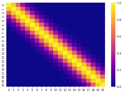
The covariance matrix is built by applying the kernels to each pairwise combination of an input variable. The kernels are special functions which take two values and compute their similarity. The overview of the commonly used kernels can be found here.
The Gaussian process is basically the generalization of a multivariate Gaussian distribution when the number of dimensions goes to infinity. In the scope of regression, each point is considered to be normally distributed so that their combined distribution is normal as well.
Similarly to the multivariate Gaussian distribution, the Gaussian process is characterized by its mean and covariance. However, the mean is not a mere vector but instead a function which can produce the mean value for an infinite number of points. And instead of covariance the kernel is used.
\[f(X) \sim \mathcal{GP}(m(X), k(XX^{T}))\]Here $m(X)$ is the mean function, and $k(XX^{T})$ is the kernel function which produces the similarity measure for each pairwise combination within $X$. Back to top ↑
Prior and posterior distribution in the Gaussian process
Without having any data from observations we may assume for example that $y$ is normally distributed over the range of $X$ variable with mean equal to 0, and variance equal to 1. We may draw a random set of points from a normal distribution which would correspond to some points in the input space $X$, and then make predictions of $y$ over unknown regions of $X$. Assuming that $y$ depends on $X$, the predictions can be made using the notion of the mean and variance of the conditional normal distribution as described above, that is using using the covariance of the input variables $X$ with themselves, and the covariance between known values of $y$ and corresponding values of $X$. In the context of Bayesian inference the resulting function distribution is considered prior distribution.
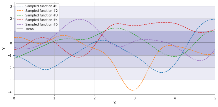
The shaded regions around the mean function correspond to the areas of one, two, and three standard deviations from the mean.
Provided that we can draw a random sample an infinite number of times - there is an infinite number of these sampled functions, and they are normally distributed around the given mean.
The prior distribution heavily depends on the kernel of choice, and its hyperparameters, because it defines the nature of relationship between variables, and thus mean and covariance of the Gaussian distribution:
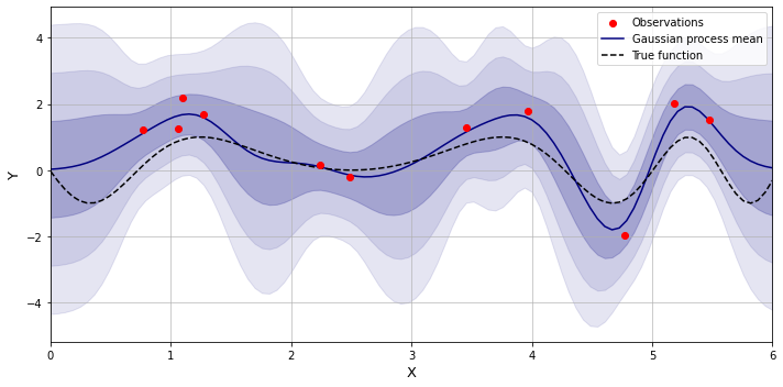
\[p_{k, \theta}(f) \sim \mathcal{N}(\mu_f, k_{ff})\]After observing some data, the function is adjusted so that it passes through the observed datapoints (or close to them), and the resulting distribution is now called the posterior. Below is an example of making predictions over unknown regions using the Gaussian process where the training points are generated using a sinusoid function with some added noise.
The posterior can be defined using the Bayes’ rule:
\[p(f \mid D) = \frac{p(D \mid f) \cdot p(f)}{p(D)} = \frac{p(D \mid f) p(f)}{\int p(D \mid f) p(f) \, df}\]where $D$ is the observed data, $p(D \mid f)$ is the likelihood function, and $p(D)$ is the marginal likelihood, that is the probability of observing the data regardless of the values which the prior assumes.
Assuming that $y$ depends on $X$, the likelihood function can be rewritten as conditional distribution $p(y \mid f(X))$, and it is also normally distributed.
\[p(y \mid f(X)) \sim \mathcal{N}(f(X), \sigma^2_n I) = \frac{1}{(2\pi)^{n/2}\det(K + \sigma^2_n I)^{1/2}} \exp \left(-\frac{1}{2} \left(y-f(x) \right)^{T}\left( K + \sigma^2_n I \right)^{-1} \left(y-f(x) \right)\right)\]Where $\sigma^2$ is the variance of the noise, and $K$ is the covariance matrix of $X$ produced by the kernel of the prior distribution.
Assuming that both the prior and the likelihood function are Gaussian, the mean and the variance of the posterior distribution can then be computed analytically in closed form using the formulas from the conditional distribution above, so there is no need for solving the integral in the denominator.
The marginal likelihood of the data can be viewed as $p(y)$. It does not depend on the particular values of $f$ but it depends on its parameters, namely its mean function $m$, and its kernel $k$ which produces the covariance matrix $K$. Thus, the distribution of the marginal likelihood is expressed as follows:
\[p(y) \sim \mathcal{N}(m(X), K+\sigma^2_n I) = \frac{1}{(2\pi)^{n/2}\det(K + \sigma^2_n I)^{1/2}} \exp \left(-\frac{1}{2} \left(y-m(x) \right)^{T}\left( K + \sigma^2_n I \right)^{-1} \left(y-m(x) \right)\right)\]Optimizing parameters
The model is believed to explain the data better if the marginal likelihood is high. Therefore, the parameters of the model (including the kernel hyperparameters) are optimized in order to maximize it.
Unlike the conditional likelihood $p(y \mid f(X))$ which depends on the prior function at each point of observation, the marginal likelihood $p(y)$ depends only on the mean of the prior distribution, so it makes it a better candidate for maximizing. Actually the log marginal likelihood is maximized because the logarithm transforms the product into the sum so that it is easier to calculate the derivative of the resulting function:
\[\log p(y) = -\frac{1}{2}(y - \mu)^T(K+\sigma^2_n I)^{-1}(y - \mu) - \frac{1}{2}\log|K+\sigma^2_n I|-\frac{n}{2}\log2\pi\]The local maximum points are found using gradient-based algorithms, such as L-BFGS-B or stochastic gradient descent, in a multidimensional space where the number of dimensions is equal to the number of the parameters.
In case of the posterior distribution above, the kernel was constructed as a sum of the squared exponential kernel and the white noise. Let’s look at the contour plot of the log likelihood dependent on two hyperparameters of the resulting kernel:
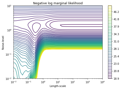
As we can see, there are at least two points of the local maxima here, so that the optimization algorithm could land at any of them. Choosing the right set of initial parameters could lead the algorithm to the desired spot of the local maxima, as well as prevent its exhaustion. Back to top ↑
Gaussian process at large datasets
When calculating the posterior mean and variance after observing $n$ datapoints, and when optimizing the hyperparameters, one has to invert a matrix of size $n \times n$, which becomes intractable for large datasets, and thus the exact calculation becomes impossible. To tackle this, sparse variational Gausian process was introduced, the idea of which is in reducing the number of dimensions from the initial dataset so that the inversion becomes tractable. While operating on a smaller dataset, we want to be able to make predictions as we would make using the posterior distribution, and for that the approximation should be as close as possible to the true posterior. The question is how to select the points which would best summarize the full dataset.
The reasonable idea is to introduce a set of $n_s$ inducing variables at some unknown locations of $X$, and a function of those variables $f_s(X_s)$ which captures the most important changes and wiggles of the underlying true function.
The number of the inducing variables is selected to be significantly smaller than the number of the observed datapoints so that it would be possible later to invert the covariance matrix of size $n_s \times n_s$. It is worth mentioning that the bigger the number of the inducing variables selected - the better the approximation, however the downside is the increased complexity of matrix inversion.
After $n_s$ is selected, the locations $X_s$ are then optimized along with the other parameters of the model, such as kernel hyperparameters, the level of noise, and the mean of the prior.
Variational inference in Gaussian process
Variational inference is the method used in the context of approximating the intractable posterior in Bayesian statistics. Here we apply it to the problem of approximating the posterior of the Gaussian process when the number of input locations is too big.
In order to find the best function $f_s$ let’s first define the marginal multivariate Gaussian distribution $q(f_s)$ with $n_s$ dimensions which captures all possible functions $f_s$.
\[q(f_s) \sim \mathcal{N}(\mu, \Sigma)\]Then let’s consider the joint distribution of $f$, which is evaluated at all training locations, and $f_s$ which is evaluated only at $n_s$ inducing locations.
\[\left(\begin{array}{c}f(X)\\ f(X_s) \end{array}\right) \sim \mathcal{N} \left(\left(\begin{array}{c} 0\\ 0 \end{array}\right), \left(\begin{array}{cc} k(X, X) & k(X, X_s) \\ k(X, X_s)^T & k(X_s, X_s) \end{array}\right)\right) = \mathcal{N} \left(\left(\begin{array}{c} 0\\ 0 \end{array}\right), \left(\begin{array}{cc} K & K_{xs} \\ K_{xs}^{T} & K_{ss} \end{array}\right)\right)\]For mathematical convenience the mean of the prior distribution is set to zero. If it is known, it may equivalently be subtracted, and then added back again when calculating the posterior (or its approximation as in our case).
The conditional distribution of $f$ provided $f_s$ is this:
\[p(f \mid f_s) = \mathcal{N}(K_{xs} K_{ss}^{-1}f_s, K - K_{xs} K_{ss}^{-1} K_{xs}^{T})\]Multiplying $p(f \mid f_s)$ by $q(f_s)$ produces the joint distribution $q(f, f_s)$ which eventually will be optimized to be the best approximation of the posterior $p(f\mid y)$. While $f$ is dependent on the choice of the hyperparameters, and the mean of the prior, $f_s$ is dependent on the inducing variables. Therefore, having both terms in the approximating distribution is crucial for the algorithm because we are aiming at not only finding the best values of the inducing variables but also optimizing the prior so that the true posterior distribution has the highest likelihood, and is good at explaining the training data.
According to variational inference approach let’s express ELBO, which is a measure that should be maximized in order to maximize to marginal likelihood $p(y)$ (our eventual objective function).
\[\text{ELBO} = \int \int \log(p(y \mid f)) q(f, f_s) \text{d}f \text{d}f_s - \text{KL}\left(q(f, f_s) \parallel p(f, f_s)\right)\]As we see, it consists of two parts: the likelihood term, and the KL divergence. We will see that both of them could be solved analytically, and thus it allows us to optimize the parameters using gradient descent.
The likelihood term after integrating out $f_s$ can be rewritten as follows.
\[\int \int \log(p(y \mid f)) q(f, f_s) \text{d}f \text{d}f_s = \int \log(p(y \mid f)) q(f) \text{d}f\]Where $q(f)$ is this:
\[\begin{aligned} q(f) &= \int q(f, f_s) \text{d}f_s = \int p(f \mid f_s) q(f_s) \text{d}f_s \\[.5em] &= \int \mathcal{N}\left(K_{xs} K_{ss}^{-1}f_s, K - K_{xs} K_{ss}^{-1} K_{xs}^{T}\right) \cdot \mathcal{N}(\mu, \Sigma) \text{d}f_s \end{aligned}\]We can see that the first multiplier relies on the values of $f_s$ but we could avoid it by factoring in the mean and the covariance of $f_s$ instead of its actual values. So,
\[\begin{aligned} q(f) &= \int \mathcal{N}\left(K_{xs} K_{ss}^{-1} \left(\mathcal{N}(\mu, \Sigma)\right), K - K_{xs} K_{ss}^{-1} K_{xs}^{T}\right) \cdot \mathcal{N}(\mu, \Sigma) \text{d}f_s \\[.5em] &= \mathcal{N}\left(K_{xs} K_{ss}^{-1} \mu, K - K_{xs} K_{ss}^{-1} K_{xs}^{T} + \left(K_{xs} K_{ss}^{-1}\right)\Sigma \left(K_{xs} K_{ss}^{-1}\right)^{T} \right) \int \mathcal{N}(\mu, \Sigma) \text{d}f_s \\[.5em] &= \mathcal{N}\left(K_{xs} K_{ss}^{-1} \mu, K - K_{xs} K_{ss}^{-1} K_{xs}^{T} + \left(K_{xs} K_{ss}^{-1}\right)\Sigma \left(K_{xs} K_{ss}^{-1}\right)^{T} \right) \cdot 1 \end{aligned}\]In the end the expression of the likelihood term in the ELBO relies on the inversion of the smaller matrix of size $n_s \times n_s$, so it is tractable. It mentions the following parameters which can be optimized:
- The parameters $\mu$ and $\Sigma$ from $q(f_s)$.
- The inducing variables (locations of the points) along with the kernel hyperparameters which produce the elements of the covariance matrix of $p(f \mid f_s)$.
- The level of noise $\sigma^2$ is mentioned in the analytical expression of $\log(p(y\mid f))$ integrated by $f$.
Speaking about the KL divergence term of the ELBO, it simplifies as follows.
\[\begin{aligned} \text{KL}\left(q(f, f_s) \parallel p(f, f_s)\right) &= \int \int \log\left(\frac{q(f, f_s)}{p(f, f_s)}\right) q(f, f_s) \text{d}f \text{d}f_s \\[.5em] &= \int \int \log\left(\frac{p(f \mid f_s)q(f_s)}{p(f \mid f_s)p(f_s)}\right) q(f, f_s) \text{d}f \text{d}f_s \\[.5em] &= \int \int \log\left(\frac{q(f_s)}{p(f_s)}\right) q(f, f_s) \text{d}f \text{d}f_s \\[.5em] &= \int \log\left(\frac{q(f_s)}{p(f_s)}\right) \left(\int q(f, f_s) \text{d}f\right) \text{d}f_s \\[.5em] &= \int \log\left(\frac{q(f_s)}{p(f_s)}\right) q(f_s) \text{d}f_s \\[.5em] &= \text{KL}\left(q(f_s) \parallel p(f_s)\right) \end{aligned}\]Which analytically solves to this:
\[\text{KL}\left(q(f_s) \parallel p(f_s)\right) = \frac{1}{2}\left[log\left(\frac{\det(K_{ss})}{\det(\Sigma)}\right) -n_s + tr\{ K_{ss}^{-1} \Sigma \} +(0 - \mu)^{T} K_{ss}^{-1} (0 - \mu)\right]\]Just like the likelihood term of the ELBO, the KL term contains the inversion of a matrix of size $n_s \times n_s$. It mentions the following parameters which can be optimized:
- The parameters $\mu$ and $\Sigma$ from $q(f_s)$.
- The inducing variables along with the kernel hyperparameters which produce the covariance matrix $K_{ss}$.
Making predictions using variational inference
After optimizing the parameters we may use the previously defined variational inference to make predictions instead of using the true posterior. Let’s define $f^{\ast}$ as a function value at testing locations. Then the conditional distribution of $f^{\ast}$ provided the data in scope of variational inference is this:
\[p(f^{\ast} \mid y) \sim \int p(f^{\ast}\mid f_s)q(f_s) \text{d} f_s\]It no longer relies on the full training dataset and uses only the inducing variables.
The term $p(f^{\ast}\mid f_s)$ is derived from the prior over the joint distribution of $f^{\ast}$ and $f_s$:
\[\left(\begin{array}{c}f^{\ast}\\ f_s \end{array}\right) \sim \mathcal{N} \left(\left(\begin{array}{c} 0\\ 0 \end{array}\right), \left(\begin{array}{cc} K_{\ast\ast} & K_{\ast s} \\ K_{\ast s}^{T} & K_{ss} \end{array}\right)\right)\]Therefore,
\[\begin{aligned} p(f^{\ast}\mid f_s) &= \mathcal{N} \left(K_{\ast s} K_{ss}^{-1} f_s, K_{\ast\ast} - K_{\ast s} K_{ss}^{-1}K_{\ast s}^{T}\right)\\[.5em] &= \mathcal{N} \left(K_{\ast s} K_{ss}^{-1} \mu, K_{\ast\ast} - K_{\ast s} K_{ss}^{-1}K_{\ast s}^{T} + \left(K_{\ast s} K_{ss}^{-1}\right) \Sigma \left(K_{\ast s} K_{ss}^{-1}\right)^{T}\right) \end{aligned}\]Then returning back to the formula of prediction, we can rewrite it as follows.
\[\begin{aligned} p(f^{\ast} \mid y) &= \int \mathcal{N} \left(K_{\ast s} K_{ss}^{-1} \mu, K_{\ast\ast} - K_{\ast s} K_{ss}^{-1}K_{\ast s}^{T} + \left(K_{\ast s} K_{ss}^{-1}\right) \Sigma \left(K_{\ast s} K_{ss}^{-1}\right)^{T}\right) q(f_s) \text{d} f_s\\[.5em] &= \mathcal{N} \left(K_{\ast s} K_{ss}^{-1} \mu, K_{\ast\ast} - K_{\ast s} K_{ss}^{-1}K_{\ast s}^{T} + \left(K_{\ast s} K_{ss}^{-1}\right) \Sigma \left(K_{\ast s} K_{ss}^{-1}\right)^{T}\right) \int q(f_s) \text{d} f_s\\[.5em] &= \mathcal{N} \left(K_{\ast s} K_{ss}^{-1} \mu, K_{\ast\ast} - K_{\ast s} K_{ss}^{-1}K_{\ast s}^{T} + \left(K_{\ast s} K_{ss}^{-1}\right) \Sigma \left(K_{\ast s} K_{ss}^{-1}\right)^{T}\right) \cdot 1 \end{aligned}\]Parametrization trick
The model that we have until now, may still not produce the best results in terms of parameters optimization. This is because the objective ELBO function has too many dimensions, and thus it may have points of local maximum which are not way different than the global one.
If we inspect the parameters of two distributions $p(f_s)$ and $q(f_s)$ we may conclude that the they are completely detached from one another:
\[p(f_s) \sim \mathcal{N}(0, K_{ss})\] \[q(f_s) \sim \mathcal{N}(\mu, \Sigma)\]Optimization of the prior with respect to the posterior happens through changing the kernel parameters, and by moving the inducing locations. At the same time the parameters $\mu$ and $\Sigma$ could be anything, and the optimizer may move them in any direction, not necessarily optimal.
One thing that can help about it is the so-called parametrization trick (whitened parameterization). Let’s define a lower triangular matrix $L$ from a Cholesky decomposition of the matrix $K_{ss}$. So to speak, $K_{ss} = LL^{T}$. Then let’s redefine $q(f_s)$ as this:
\[q(f_s) = \mathcal{N}(L\mu, L\Sigma L^{T})\]This links together $p(f_s)$ and $q(f_s)$ so that optimization of the kernel parameters leads to changes within $q(f_s)$ as well. In practice this achieves better approximation of the posterior because the optimizer is better directed towards the point of the local maximum.