Correlation and variance in linear regression

What is covariance?

Covariance is a measure of the joint variability of two random variables. If the greater values of one variable mainly correspond with the greater values of the other variable the covariance is positive. In the opposite case, when the greater values of one variable mainly correspond to the lesser values of the other variable, the covariance is negative. The magnitude of the covariance is not easy to interpret because it is not normalized and hence depends on the magnitudes of the variables. That is, high absolute values will lead to a higher magnitude of covariance.

Calculation of covariance is very similar to the calculation of distribution variance, however instead of squaring the difference we take a product of differences of both variables from the mean.

     $Cov(X,Y)$ = $\frac{1}{n-1}\sum_{i=1}^n (x_i-\overline{x})(y_i-\overline{y})$

In the denominator we have $(n-1)$ instead of just $n$ in order to account for the variance of the sample mean. More to it can be found here).

For multiple variables it is possible to calculate the covariance matrix which contains all covariance values of all pairwise combinations of the variables. It’s a square symmetric matrix with the diagonal elements equal to the variance of corresponding variables.

\[C = \frac{1}{n-1}\sum_{i=1}^n (x_i - \bar x)(x_i - \bar x)^{T} = \left[\begin{array}{cccc} Var(x_{1}) & Cov(x_1, x_2) & ... & Cov(x_1, x_m) \\ Cov(x_2, x_1) & Var(x_{2}) & ... & Cov(x_2, x_m) \\ ... & ... & ... & ... \\ Cov(x_m, x_1) & Cov(x_m, x_2) & ... & Var(x_{m}) \end{array} \right]\]

If the variables in each vector of a matrix are centered around their respective mean values then the covariance matrix can be calculated just like this:

     $C = \frac{1}{n-1}X^{T}X$

What is correlation?

Correlation coefficient (also known as Pearson’s correlation coefficient) is a standardised (or scaled) version of covariance. Generally speaking correlation is a measure of how two variables are related. Increase of one variable may cause another to increase or decrease and vice versa. In linear regression with two variables we use correlation coefficient in order to understand how well a line describes the relationship between them.

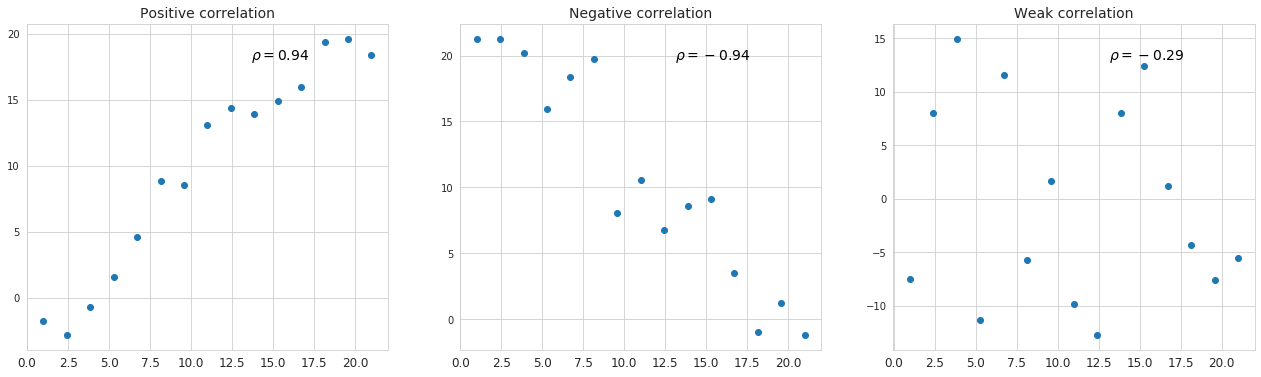
     $\rho_{X,Y} = \frac{Cov(X,Y)}{\sigma_X \sigma_Y}$

The value of correlation coefficient lies between -1.0 and 1.0. If correlation coefficient equals 1 then the upward sloping line can completely describe the relationship. And vice versa, if the correlation coefficient equals -1 then the relationship can be completely described with the downward slope. And if the correlation coefficient is close to 0 then the line is not describing the relationship well at all.

Below is representation of different kinds of simple linear regression where correlation coefficient assumes different values.

Coefficient of determination

A related concept to correlation with regard to the linear regression is the coefficient of determination, also known as $R$-squared. This coefficient represents the strength of linear relationship in the model by measuring how much of the variation in the dependent variable is caused by independent variables.

The predicted value $\hat Y$ constitutes the range of variance which is explained by independent variables while the observed value $Y$ represents the total variance which consists of the variance of $\hat Y$ and the variance of the error term $\varepsilon$. From here the coefficient of determination is the ratio of explained variance to the total observed variance.

     $R^2 = \frac{\sum_{i=1}^n(\hat y_i - \bar y)^2}{\sum_{i=1}^n(y_i - \bar y)^2} = 1 - \frac{\sum_{i=1}^n \varepsilon_i^2}{\sum_{i=1}^n(y_i - \bar y)^2}$

The latter expression is obtained from the assumption that the mean of the error term is 0.

An alternative way to think of the coefficient of determination is to imagine the squared version of the correlation coefficient which measures the relationship between observed and predicted values of the dependent variable. This actually explains where the “squared” part in the term “$R$-squared” comes from.

     $\rho = \frac{\frac{1}{n}\sum_{i=1}^n(y_i-\bar y)(\hat y_i - \bar y)}{\sqrt{(\frac{1}{n}\sum_{i=1}^n(y_i-\bar y)^2)(\frac{1}{n}\sum_{i=1}^n(\hat y_i - \bar y)^2)}} = \frac{Cov(Y, \hat Y)}{\sqrt{Var(Y)Var(\hat Y)}} = \frac{Cov(\hat Y + \varepsilon, \hat Y)}{\sqrt{Var(Y)Var(\hat Y)}} = \frac{Cov(\hat Y, \hat Y) + Cov(\hat Y, \varepsilon)}{\sqrt{Var(Y)Var(\hat Y)}}$

Assuming that there is no correlation between the predicted values and the error term, the expression above transforms into this:

     $\rho = \frac{Var(\hat Y)}{\sqrt{Var(Y)Var(\hat Y)}}$

And the squared version:

     $\rho^2 = \frac{Var(\hat Y)}{Var(Y)} = R^2$

On the whole, higher values of the coefficient of determination mean tighter distribution of observed values around the predicted ones with little noise, so this generally indicates a good fit. However this alone does not prove that the selected model was built correctly, and that there is no bias in it. There still might not be enough data, the predictors might be poorly selected, be collinear or not have an impact on the dependent variable.

Adjusted R-squared

The standard version of $R$-squared has a particular property which often makes it less suitable for analysis - namely it always increases if new variables are added to the model, regardless whether they are meaningful or not. This is why we may end up with a high value of $R$-squared when in fact the predictors poorly describe the dependent variable. In the extreme situations when the number of variables is equal to the number of observations we’ll have a system of linear equations the parameters of which make an exact fit of the modeled values to the observed ones, and $R$-squared will be equal to 1.

In order to deal with this shortcoming, an enhanced version of the coefficient of determination was introduced - the adjusted $R$-squared. It penalizes $R$-squared with the number of independent variables decreasing the degree of freedom.

     $\bar R^2 = 1-(1 - R^2)\frac{n-1}{n-p-1}$

where $n$ is the number of observations, and $p$ is the number of independent variables. $(n-1)$ is the number of degrees of freedom of the total variance in the model (1 is subtracted because the mean value used for calculation of the total variance is estimated from the sample. More to it can be found here), and $(n-p-1)$ is the number of degrees of freedom for the variance of the error term.

The adjusted $R$-squared is never greater than the vanilla $R$-squared, and it actually decreases if meaningless variables are added to the model.

Variance of coefficients in linear regression

One of the core assumptions in the linear regression is the normal distribution of the error term around the mean value of 0. According to this, the coefficients in the model are random values as well, and their means are found via least squares. This corresponds with the fact that for a different sample of observations the estimated coefficients are different. From here it is reasonable to estimate the variance of coefficients in order to derive their standard errors and confidence intervals. Below is some intuition on how the formula for the variance of coefficients in the linear regression is obtained.

Recall that $\hat \beta = (X^{T}X)^{-1}X^{T}Y$, and $Y = X \beta + \varepsilon$, where $\beta$ is the true value of coefficients, and $\hat \beta$ is the estimate. The general formula for variance in matrix form is this:

     $Var(A) = E[AA^{T}]-E[A][E[A]]^{T}$

Using it we build a formula for the variance-covariance matrix of $\hat \beta$:

\[Var[\hat \beta] = E[((X^{T}X)^{-1}X^{T}Y)((X^{T}X)^{-1}X^{T}Y)^{T}] - E[\hat \beta][E[\hat \beta]] \\ = E[((X^{T}X)^{-1}X^{T}(X \beta + \varepsilon))((X^{T}X)^{-1}X^{T}(X \beta + \varepsilon))^{T}] - \beta^2 \\ = E[((X^{T}X)^{-1}X^{T}X \beta + (X^{T}X)^{-1}X^{T}\varepsilon))((X^{T}X)^{-1}X^{T}X \beta + (X^{T}X)^{-1}X^{T}\varepsilon))^{T}] - \beta^2 \\ = E[(\beta + (X^{T}X)^{-1}X^{T}\varepsilon))(\beta + (X^{T}X)^{-1}X^{T}\varepsilon))^{T}] - \beta^2 \\ = \beta^2 + E[((X^{T}X)^{-1}X^{T}\varepsilon)((X^{T}X)^{-1}X^{T}\varepsilon)^{T}] - \beta^2 \\ = E[(X^{T}X)^{-1}X^{T}\varepsilon \varepsilon^{T}X(X^{T}X)^{-1}] = \sigma^2 (X^{T}X)^{-1}\]

Where $\sigma^2$ is the variance of the error term. The diagonal elements of the resulting matrix represent the variance of the coefficients.

From this we make a conclusion that the variance of coefficients is bigger in noisy datasets. At the same time, the variance decreases if the spread in $X$ increases which makes sense, since increasing the range of possible values of independent variables reduces the effect of the noise, and according to the Central limit theorem, the distribution of the error term and the parameters start to resemble normal distribution.

Variance inflation factor

Variance inflation factor (VIF) is a measure of variance of a coefficient in a linear regression which is caused by multicollinearity. This indicator is calculated separately for each independent variable in the model by building a regression where this variable is described by other independent variables (the dependent variable is omitted here). Looking at the coefficient of determination for the built regression it is possible to get the idea of how much the variance of the variable is determined by other variables, and it also serves as an indicator of multicollinearity. Now let’s take a look at the how VIF is constructed:

     $VIF_i = \frac{1}{1-R_i^2}$

If there is no multicollinearity for a given variable VIF will assume the value of 1, otherwise it will be higher. Compared to $R$-squared the variance inflation factor has one additional statistical property - it provides a numerical measure of how much the variance of coefficient is inflated due to multicollinearity (just like the name suggests). For practical reasons values of VIF higher than 5 (this corresponds to the values of $R$-squared higher than 0.8) indicate multicollinearity.