Statistical distributions
A set of discrete values or a range of continuous values of a random variable is characterized by a certain probability distribution. In statistics various distributions arise in the context of estimating probabilities of random values or events.
In case of discrete variables the distribution is described by the probability mass function (PMF) which assigns a certain probability value for each individual value from the set. For continuous random variables, probability density functions (PDF) provide values of relative likelihood of assuming a certain value. Although the probability that a continuous variable will assume a certain exact value is 0, PDF allows to compare the relative likelihoods in different ranges of values, as well as to calculate the probability of assuming a value within a specific range (using integral calculus).
In this article the most useful probability distributions will be explained, as well as some of the distributions which derive from them.
Normal distribution
Normal distribution (also known as Gaussian distribution) is one of the most fundamental building blocks of statistics. According to the Central limit theorem, averages of random samples, which are drawn independently from some independent distribution converge around some central value. They become normally distributed when the number of observations is sufficiently large. At this point the distribution of the original values from which the samples are drawn doesn’t even have to be normally distributed.
Suppose, we decided to measure the weight of all newborns in a multitude of different hospitals and calculate the average weight in each hospital. Most likely the distribution of those average weights will resemble a bell-shaped curve.
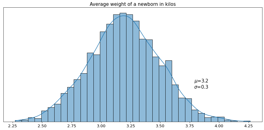
Here we see that the average of all measured averages converges around a certain central value, 3.2 kilos in this case. This means that among all measured averages we encountered mostly values which are very close or equal to 3.2. The closer the hospital average to 3.2 - the higher the frequency of such encounters. By contrast, we see that there are very few averages that have values, say, higher than 4 or lower than 2.5 kilos. The bell-shaped function that we have above is actually the approximation of probability density function for the given distribution, and its values provide relative likelihood of a random variable (in our example the weight of the newborn) to assume certain values.
Normal distribution has nice statistical properties, with regard to probability in particular. From the example above we can see that we have a 50% chance of getting an average newborn weight higher or lower than 3.2 kilos, whereas the whole area under the curve represents 100% of the overall probability.
One other interesting property of normal distribution is the spread of its values around the mean, known as the six sigma rule.
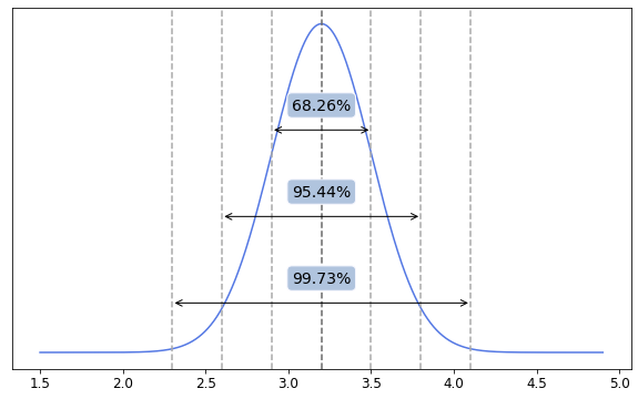
Based on the example above, we may deduce that:
- 68.26% of all newborns have weight from 2.9 to 3.5 kilos (one standard deviation away from the mean)
- 95.44% - from 2.6 to 3.8 kilos (two standard deviations away from the mean)
- 99.73% - from 2.3 to 4.1 kilos (three standard deviations away from the mean)
Before moving on to calculating the probability of getting certain interval values, let’s introduce the $z$-score metric. Plainly speaking, $z$-score tells us how many standard deviations a given value is away from the mean of its distribution.
$z = \frac{x-\mu}{\sigma}$
In general, in order to calculate the area under the curve we would have to perform integral calculus, however for the normal distribution we can simply use precalculated $z$-table by looking up probability for a specific $z$-score. $Z$-table has recorded values of integral for cumulative normal distribution function, and it shows the probability of a random variable to assume value less than some other value. There are two parts of $z$-table - for $z$-scores which are higher or lower than the mean of distribution.
Suppose we want to calculate the percentage of newborns who have weight less than 3 kilos and the percentage of newborns with weight from 3 to 3.5 kilos. That is equal to calculating the filled areas under the curves below.
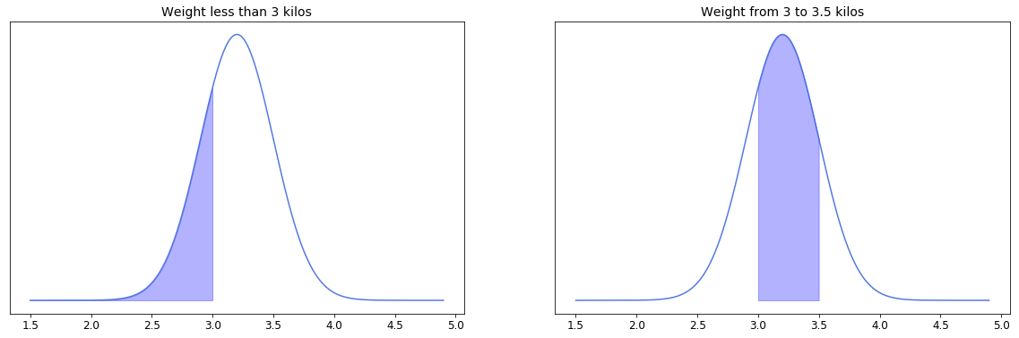
In the first case we simply calculate $z$-score of the value 3 and look up the area under the curve from the $z$-table for negative values (since 3 is lower than the mean 3.2). In this example it approximates to 0.2514. So conclude that only 25.14% of all newborns have weight 3 kilos or less.
In the second example we have an area with two cut-off points. $Z$-table allows us to find the area to the left from a specific value, so here is what we do. First we calculated $z$-scores for 3.5 and for 3, then we looked up the area under the curve for all weights which are less than 3.5 kilos and those which are less than 3 kilos. Then we simply subtract the second from the first. Finally we end up with something like 0.8413 - 0.2514, which equals 0.59. Here we conclude that nearly 59% of all newborns have weight between 3 and 3.5 kilos.
The probability density function of the normal distribution which was used in construction of $z$-table, and which is generally used for calculating probability looks like this:
$f(x) = \frac{1}{\sigma\sqrt{2\pi}}e^{-\frac{1}{2}(\frac{x-\mu}{\sigma})^2}$ Back to top ↑
Student’s t-distribution
If there is a need to estimate the mean of population using a sample, and if the population’s variance is unknown then the mean of the population itself becomes random variable with its own variance. As a consequence, the estimated variance of the population becomes higher than just the variance of the sample.
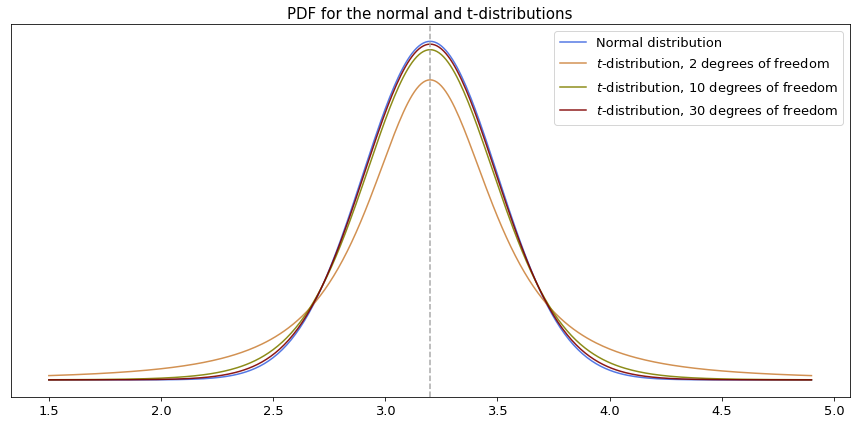
Student’s distribution (or $t$-distribution) is used as the probability density function for the expected value of population based on the sample statistics. This type of distribution is very similar to the normal distribution but it has thicker tails if the number of samples is small (roughly less than 30), and thus values which are more distant from the sample mean have higher probability of occurring. On the other hand, if the size of a sample goes to infinity then the $t$-distribution converges to the normal distribution. The shape of the PDF is actually defined by the number of degrees of freedom of the distribution, which is the same as for the estimated variance - namely $(n-1)$, where $n$ is the number of observations in the sample. Below is a comparison of probability density functions with different numbers of degrees of freedom for the same example of the newborn weight which we used earlier.
Similarly to $z$-scores for the normal distribution, for $t$-distribution there are also tables of precomputed values for different numbers of degrees of freedom, so no need to perform integration when calculating probability. Back to top ↑
Studentized range distribution
This type of distribution is used in hypothesis testing when the means of more than two samples are tested for being equal (whether or not all samples come from the same normal distribution).
If multiple samples of the same size are drawn from the same population then the following statistic will follow the studentized range distribution:
$q = \frac{\bar x_{max} - \bar x_{min}}{\frac{s}{\sqrt{n}}}$
where $\bar x_{max}$ and $\bar x_{min}$ are the largest and the smallest means of the samples, $s$ is the pooled standard deviation, and $n$ is the sample size. The number of degrees of freedom is selected as for the pooled variance: $k$($n$-1), where $k$ is the number of groups.
If the $q$-statistic exceeds the critical value of the distribution for a given number of samples and degrees of freedom, then the null hypothesis that the two sample means are from the same normal distribution is rejected.
The studentized distribution depends on both the number of samples and the number of degrees of freedom. The more samples - the higher probability that the difference between the largest and the smallest means is due to chance. Therefore, the critical value becomes larger as the number of samples increases.
Chi-square distribution
In a nutshell the chi-square distribution is the distribution of sum of squared values sampled from a normally distributed variable.
$\chi_k^{2} = \sum_{i=1}^k Z_i^2$
where $Z_i$ is a randomly drawn value from a normal distribution, and $k$ is the number of degrees of freedom, which is also equal to the number of drawn values.
Below is a visualization of the probability density function of the chi-square distribution for a different number of degrees of freedom if the values are drawn from the normal distribution with the mean value 0, and the standard deviation 1.
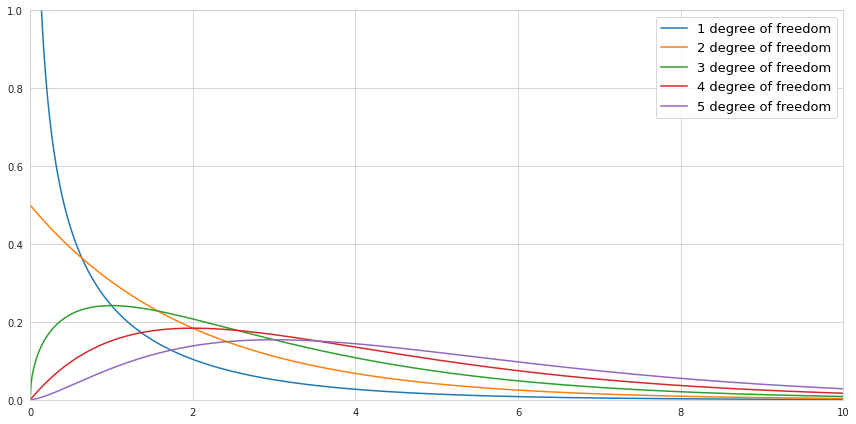
Notice that since we are squaring the values there are no negative values in the chi-square distribution. If we draw only one value, then there is a high probability that this value is close to 0, since the normal distribution is centered around 0. Therefore the shape of the PDF of chi-square distribution with 1 degree of freedom is heavily skewed towards zero, while the probability of getting bigger numbers becomes minuscule. If we draw more and more numbers increasing the number of degrees of freedom, the sum of squared values causes the center of the PDF of chi-square distribution to be shifted to the right. Back to top ↑
Binomial distribution
This distribution is used for getting probabilities in a discrete random variable which consists of Bernoulli trials (or experiments) - observations the end results of which are restricted to only two possible outcomes. The most commonly referred example of a Bernoulli trial would be tossing of a coin and expecting the outcome to be either heads or tails. However, in fact any variable may be translated into a Bernouli trial, even a continuous one. For example we may consider one of the possible outcomes as a success, and all the rest as a failure. For continuous variables we may specify a threshold, and then consider the outcomes as crossing or not crossing it.
A random variable follows binomial distribution if it represents the number of successes in a sequence of Bernoulli experiments. The probability mass function is constructed using the knowledge of probability of success in a single experiment:
$f(x) = {\binom{n}{x}}p^{x}(1-p)^{n-x}$
where $p$ is a probability of success in a single experiment, $x$ is the number of expected successes, $n$ is the number or experiments, and where
$\binom{n}{x} = \frac{n!}{x!(n-x)!}$
The assumptions of this type of distribution are independence of each observation and the same probability of success for each individual Bernoulli trial.
In order to achieve better accuracy with binomial distribution testing the whole experiment may be performed multiple times (or the observations may be resampled with replacement). For example we want to estimate how well the audience likes a new movie. The outcome for each individual cinema visitor is viewed as a Bernoulli trial while the number of satisfied visitors after a session is the result of a single binomial test. Since this measure itself may depend on many factors the results after each session may be quite different. In order to understand the average percentage of the audience satisfaction it may be useful to visualize with a histogram the total number of outcomes for the binomial tests across all sessions. Below is a plot displaying distribution of binomial test results for 1000 sessions each containing 200 visitors.
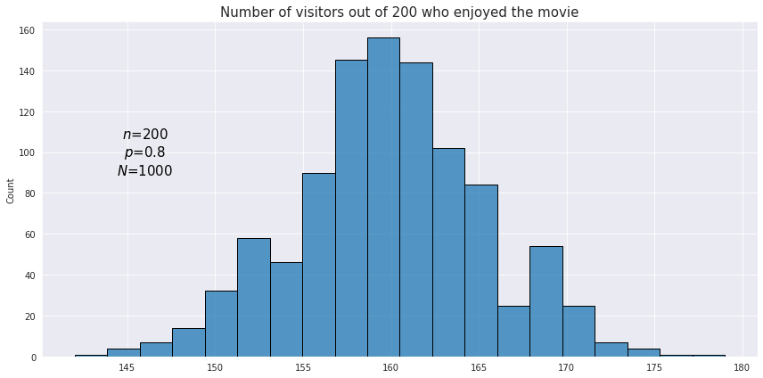
As we see just like in the normal distribution the resulting values are concentrated around a certain central value - the mean of the binomial distribution. In fact, if the number of tests is reasonably high (at least both $np$ and $n(1-p)$ are greater than 5) then the binomial distribution may be approximated with the normal distribution.
Let’s set the value of success as 1, and the value of failure as 0. Then the probability of 1 is $p$ while the probability of 0 is $(1-p)$. The weighted average of a single experiment will be:
$E(x) = 1 \cdot p+0 \cdot (1-q) = p$
From this the expected value (or the mean) of the distribution is simply $np$.
Now let’s recall that the variance measures the sum of squared distances between the observed and expected values of a random variable. For a successful outcome of a Bernoulli trial where we have 1, the distance to the mean ($p$) will be $(1-p)$. Similarly, for the unsuccessful outcome where we have 0 the distance to the mean will be $(0-p)$. Then the weighted average of these two will be:
$Var(x) = p(1-p)^2+(1-p)(0-p)^2 = p(1-p)^2+(1-p)p^2 = p(1-p)(1-p+p) = p(1-p)$
Therefore the variance for the binomial distribution is $np(1-p)$. Back to top ↑
Geometric distribution
This is a type of distribution which is used to model the number of failures in sequences of Bernoulli trials before the first success (or vice versa). For example we want to know how many customers a retail shop has to engage with before the first sale is made.
The PMF of the geometric distribution is given by the following formula:
$f(x) = (1-p)^{x} p$
The formula is pretty intuitive as it just calculates the joint probability of $x$ failures in Bernoulli trials, each having probability of $(1-p)$, and 1 success probability of which is $p$.
Below is an example of what an observed geometric distribution could look like:
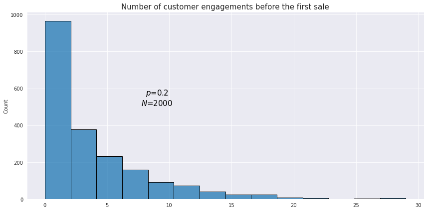
From our example above the probability of having the first successful sale after 2 unsuccessful customer engagements would be
$f(2) = (1-0.2)^{2} \cdot 0.2 = 0.128$
The mean of the geometric distribution is defined as $\frac{1-p}{p}$, and the variance is $\frac{1-p}{p^2}$. Back to top ↑
Negative binomial distribution
This distribution is the generalization of the geometric distribution which is used to model the number of failures before the $n$th success. The PMF is the following:
$f(x; r) = \binom{x+r-1}{r-1}(1-p)^{x}p^r$
where $r$ is the required number of successes, $p$ is the probability of a success in a single Bernoulli experiment, and where
$\binom{x+r-1}{r-1} = \frac{(x+r-1)!}{(r-1)!x!}$
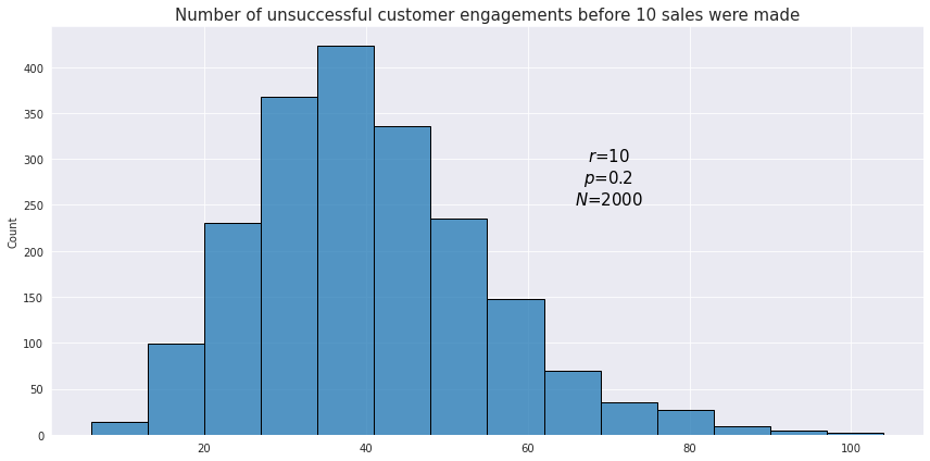
Using the same example as with the geometric distribution, let’s see how the distribution looks like for the number of unsuccessful customer engagements before 10 sales were made.
The mean of the negative binomial distribution is defined as $\frac{pr}{(1-p)}$, and the variance is $\frac{pr}{(1-p)^2}$.Back to top ↑
Beta distribution
This distribution is an extension of the negative binomial distribution to the continuous variables. However, instead of modeling the number of successes (or failures), it is used for modeling the distribution of probability.
Let’s imagine that out of 100 customers who went to a gym trial, only 63 decided to buy an annual membership. How would one describe the probability of purchasing a gym membership after trying a trial? The most obvious answer would be say 63%, and this is not wrong, yet it might be useful to resort to a distribution instead of picking just one number for probability. See, 63% is the statistic of a sample, and the true percentage might be different. As such, we might want to know the probability that the true probability of buying a gym membership is greater than 50% for example. This is where the beta distribution comes to rescue because using its probability density function we can simply integrate over all its values higher than 0.5.
The beta distribution is defined for the inclusive range between 0 and 1, and its PDF looks like this:
$f(x; \alpha, \beta) = \frac{x^{\alpha -1}(1-x)^{\beta -1}}{\mathrm{B}(\alpha, \beta)}$
where $\alpha$ and $\beta$ reflect the proportion of successes and failures accordingly, and $\mathrm{B}(\alpha, \beta)$ is a normalization coefficient defined as follows:
$\mathrm{B}(\alpha, \beta) = \frac{\Gamma(\alpha)\Gamma(\beta)}{\Gamma(\alpha+\beta)}$
The gamma-function $\Gamma$ is an extension of the factorial expression to complex numbers which makes it possible to use it for a continuous range of numbers.
$\Gamma (n) = (n-1)! = \int_{0}^{\infty} x^{n-1}e^{-x} dx$, for $n$ > 0
Now, when we look at the formula of the PDF of the distribution more closely, we can see that it is very similar to the PMF of the negative binomial distribution. Since the beta distribution is continuous, the binomial coefficient from the binomial distribution is replaced with the expression which consists of the gamma functions:
$\binom {n}{k} = \frac {n!}{k!(n-k)!} = \frac{\Gamma(n+1)}{\Gamma(k+1)\Gamma(n-k+1)} = \frac{1}{\mathrm{B}(k+1, n-k+1)}$
Below we can see how the probability density function of the beta distribution would look like depending on the choice of the parameters.
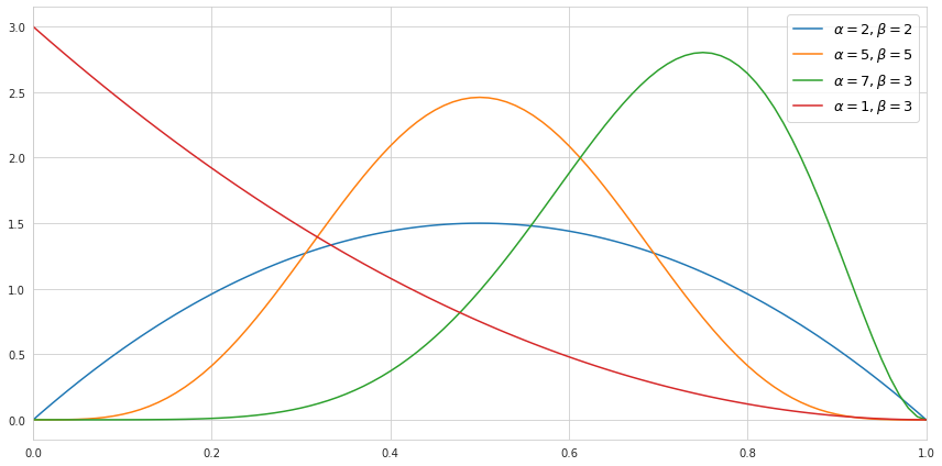
It is worth mentioning that the higher the value of the parameters - the tighter the values are centered around its mean, which reflects the certainty about the distribution.
The mean of the beta distribution is defined as $\frac{\alpha}{(\alpha+\beta)}$, and the variance is $\frac{\alpha\beta}{(\alpha+\beta)^2(\alpha+\beta+1)}$. Back to top ↑
Uniform distribution
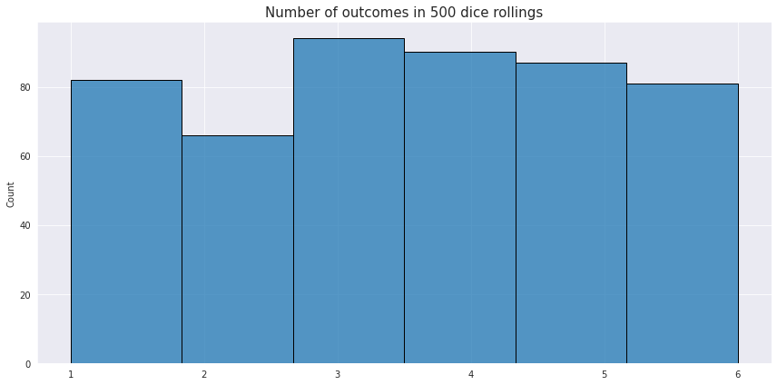
This type of distribution describes processes where every possible outcome has the same chance of occurring. An example of a discrete uniform distribution is rolling of a dice once and expecting any of the possible 6 values. Random number generation is an example of a continuous uniform distribution.
The PMF for the discrete distribution is just $\frac{1}{n}$, where $n$ is the number of partitions with the equal probability. For the continuous distributions the PDF is a constant line:
$f(x) = \frac{1}{b-a}$
where $a$ and $b$ are the borders of the distribution.
The expected value of the uniform distribution is defined as the center of the range over which the value is distributed $\frac{a+b}{2}$. For the discrete distribution the variance is calculated as $\frac{n^2-1}{12}$ while for the continuous distribution as $\frac{(b-a)^2}{12}$. Back to top ↑
Poisson distribution
This distribution is used to model the number of events which occur during a fixed period of time, for example the number of customer complaints per month or the number of trains arriving during a certain hour. Similarly to the binomial distribution, all occurrences of events are considered random and independent, so the occurrence of one event does not affect the probability of another event.
The probability mass function of the Poisson distribution uses prior knowledge of the average number of occurrences per period - parameter $\lambda$. This parameter can actually be derived from the binomial distribution as $\lambda = np$, where $p$ is the probability of a single event occurrence, and $n$ is the number of Bernoulli trials. Both mean and variance of a random variable which follows the Poisson distribution are equal to $\lambda$, and this is the formula of its PMF:
$f(x; \lambda) = \frac{\lambda^{x}e^{-\lambda}}{x!}$
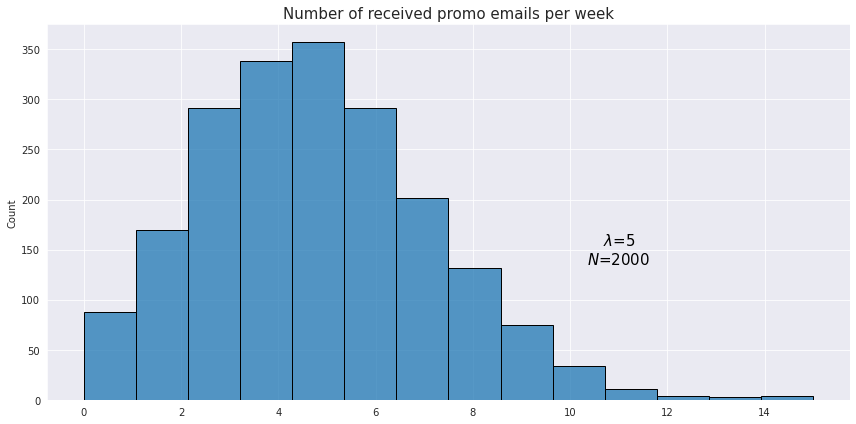
For example, a person receives on average 5 promotional emails from different sellers. The probability of receiving 3 emails would be
$f(3; 5) = \frac{5^{3}e^{-5}}{3!} \approx 0.14$
Here is an example of an observed distribution of the number of received emails for a sample of 2000 users.
Exponential distribution
This is a continuous distribution which is closely related to the Poisson distribution as it models the time between random independent events. It may also be viewed as a continuous analogue of the geometric distribution. The PDF of the distribution is calculated as follows:
$f(x; \lambda) = \lambda e^{-\lambda x}$
Suppose we would like to model the time between arrival of two buses at some station when on average there are 4 incoming buses for an hour. Translating this into minutes we have $\lambda = \frac{4}{60} \approx 0.07$. This is what a hypothetical distribution of time in minutes would look like:
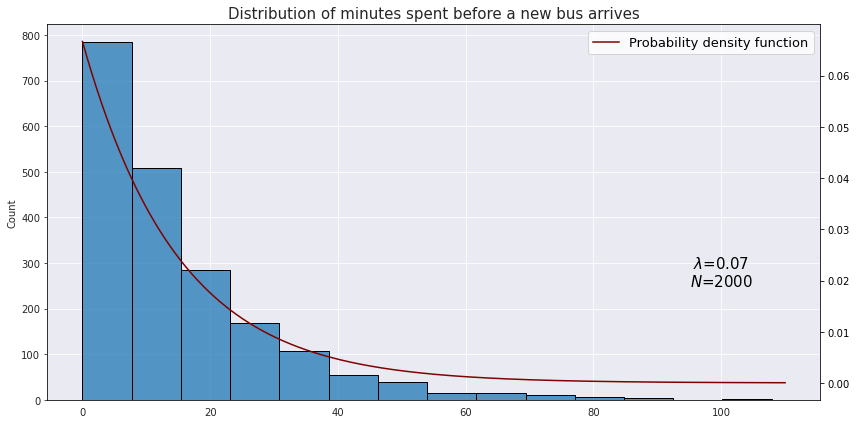
The mean of the exponential distribution is $\frac{1}{\lambda}$, and the variance is $\frac{1}{\lambda^2}$. Back to top ↑