Sampling distribution
In real life situations it is often impossible to calculate statistics such as mean and variance for the whole population. Instead we may only be able to draw a sample from the whole population, calculate statistics over it, and project it on the whole population. Of course, sample statistics won’t correspond fully to that of the whole population, and it may vary among different samples, since each sample is drawn independently. From here, a definition of sampling distribution arises, which is the probability distribution of sample statistics.
In this article
- Sample mean
- Sample variance vs estimation of the true variance
- Confidence interval and margin of error
Sample mean
Expectation of the sample mean
As stated above, if we randomly draw $n$ samples from the population and calculate the mean value of each, we’ll likely get different results. Here, the mean of a sample (signed as $\bar X$) becomes a random variable. Yet it is possible to calculate the expected value of $\bar X$ (in other words the mean of the sample mean), and its variance. For the expected value we have:
$E[\bar X] = E[\frac{x_1 + x_2 + … + x_n}{n}] = \frac{1}{n}E[x_1 + x_2 + … + x_n] = \frac{1}{n}(E[x_1] + E[x_2] + … + E[x_n])$
The expectation of each of the individually drawn values is equal to the mean of the population $\mu$, so:
$E[\bar X] = \frac{1}{n}(\mu + \mu + … + \mu) = \frac{n \mu}{n} = \mu$
Eventually the expected value of the sample mean is equal to the mean of the population.
Interestingly, the distribution of means of different independently drawn samples tend to resemble normal distribution as the number of samples increases. This phenomenon is known as the Central limit theorem and it applies to any type of population distribution. Back to top ↑
Variance of the sample mean
Before moving to the expression of the variance of the sample mean it is worth to mention that the constant is getting squared after moving from the expression of variance:
$Var(aX) = E[(aX - E[aX])^2] = E[(aX - aE[X])^2] = E[a^2(X - E[X])^2] = a^2 E[(X - E[X])^2] = a^2 Var(X)$
Remembering this, we can calculate the variance of the sample mean:
$Var(\bar X) = Var(\frac{x_1 + x_2 + … + x_n}{n}) = \frac{1}{n^2}Var(x_1 + x_2 + … + x_n) = \frac{1}{n^2}(Var(x_1) + Var(x_2) + … + Var(x_n))$
The variance of each of the individually drawn values is equal to the variance of the population $\sigma^2$, so:
$Var(\bar X) = \frac{1}{n^2}(\sigma^2 + \sigma^2 + … + \sigma^2) = \frac{n \sigma^2}{n^2} = \frac{\sigma^2}{n}$
The variance of the sample mean is much less than the variance of the population which means that the sample mean won’t be much different in different independently drawn samples. Taking into consideration the Central limit theorem, it makes sense because the sample mean will tend to be near the true mean as the number of samples increases.
The equivalent of standard deviation for sample distribution is called standard error which essentially is the estimate of the error of making assumptions about the true mean.
$SE = \frac{\sigma}{\sqrt{n}}$
where $\sigma$ is the standard deviation in the sample. Back to top ↑
Sample variance vs estimation of the true variance
It should be stated that the sample variance is not quite the true representative of the population’s variance, since we usually know only the expectation of the true mean (the mean of the sample) but not the true mean itself. As was discussed in the previous section, the sample mean has its own variance which is equal to the true variance divided by the number of samples. Thus, the true variance will have to incorporate this metric, as well as the variance of the sample.
$\sigma^2 = \hat{\sigma^2} + \frac{\sigma^2}{n}$
where $\hat{\sigma^2}$ is the sample variance which we can directly calculate using the sample mean. By little rearrangement we have:
$\hat{\sigma^2} = \sigma^2 - \frac{\sigma^2}{n} = \sigma^2 \cdot \frac{n-1}{n}$
From this we get the unbiased estimate of the true variance:
$\sigma^2 = \frac{\hat{\sigma^2}}{\frac{n-1}{n}} = \frac{\sum_{i=1}^n(x_i-\bar x)^2}{n-1}$ Back to top ↑
Confidence interval and margin of error
Using the notion of standard error of the sample mean, for a certain confidence level it is possible to define the bounds for the region where the true mean might be - the confidence interval. Depending on the sample mean different samples may produce different confidence intervals, therefore the confidence level is the probability that a randomly drawn sample will produce a confidence interval containing the true mean. A common misconception is that the confidence level is the probability that the true mean lies within a certain confidence interval.
The confidence interval is expressed as the region around the point estimate of the mean:
$(\bar X - Z \cdot SE; \bar X + Z \cdot SE)$
where $Z$ is the critical value for a given significance level (confidence level minus 1). For the normal distribution the $z$-value tells how many standard deviations from the mean a certain value is. $Z$-value can be used if it is assumed that the population has normal distribution, and if its standard deviation is known. If the population’s standard deviation is unknown, it is estimated from the sample, as described in the previous section, only in this case $t$-value is used instead of $z$-value. In addition, $t$-value is typically used if the size of the sample is less than 30. While $z$-value follows normal distribution with the mean value of 0, $t$-distribution has similar shape but with thicker tails so under the same significance level it allows the test statistic to stray further from the true mean. At any rate, for a certain significance level it is possible to get $z$- or $t$-statistic from a table of precomputed values. When estimating the confidence interval, the table for the two-tailed distribution should be used, as the area of the smallest probability is located to the both sides of the mean estimation. Below is the distribution plot of a confidence interval.
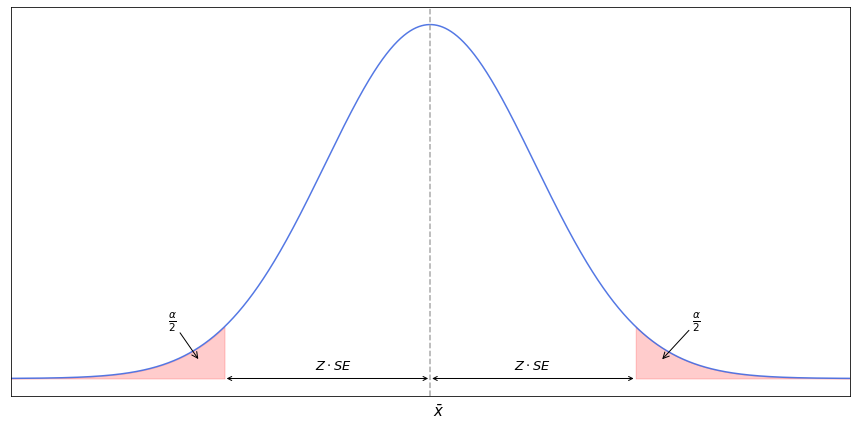
As we see, the area covered by the significance level is split in halves and occupies the farthest regions of the distribution.
The expression $z \cdot SE$ is the margin of error, and it depends only on the populations’s standard deviation, number of the samples, and the selected confidence level. It does not depend on the mean of the sample, hence we get different confidence intervals for the different samples of the same size when their mean values are different. Back to top ↑