Hypothesis testing
In this article
- What is hypothesis testing
- P-value hacking
- Type I and type II errors
- Statistical power
- Power analysis
- Multiple hypothesis testing
What is hypothesis testing
In a nutshell hypothesis testing is a process of validation of plausibility of an assumption about population data using sample data. The assumption which is being tested is called the null hypothesis. Alongside the null hypothesis the alternative hypothesis is defined as rejection of the null hypothesis.
Under the framework of hypothesis testing we assume that the null hypothesis is true, calculate statistic over the sample data (sample mean for example), and evaluate the probability of having this (or more extreme) statistic if the null hypothesis is true, which is called $p$-value. If the probability is greater then some threshold (the significance level), then the hypothesis is not rejected. On the other hand, if the probability of getting that sample statistic under the null hypothesis is small (smaller than the significance level), then it is rejected and the alternative hypothesis is assumed.
One important consideration about $p$-values is that it reflects probability of getting a statistic at least that extreme as we got from a sample. In other words, if a sample produces a statistic of value $x$ then the $p$-value shows probability of getting exactly $x$ or other values which are more rare then $x$.
In the following illustration we see that for some distribution of a random variable, the $p$-value covers an area of probability smaller than the area covered by the significance level, hence the hypothesis is rejected.
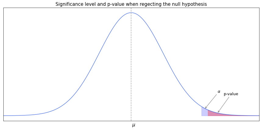
As a rule, the null hypothesis is the hypothesis of no change. For example we assume that the mean value of some distribution of a random variable is equal to some number, or that the mean values of two distributions are equal, or that the proportion of the population is equal to some percentage. The alternative hypothesis may suggest that the statistic is either greater or smaller than the one in the null hypothesis - in this case we have a one-tailed test (as in the picture above). Or it may suggest that the statistic is not equal to the one in the null hypothesis (varying in either direction) - then we have a two-tailed test. In case of two-tailed tests the probability area of significance level area is split into halves and placed on either side of the mean.
Depending on the type of hypothesis testing a different test statistic is used. The choice depends for example on whether the difference is tested between a sample and the population, or between two or samples. Also we might be testing the difference in means, the difference in variance or the difference in discrete value distributions, which would also affect the choice of test statistic. Back to top ↑
P-value hacking
$p$-value hacking is associated with making incorrect decisions based on test statistics when the desired outcome is made to look true based on the significance test. Since the significance level implies the chance to reject the null hypothesis when it is true, one might be tempted to draw multiple tests from the same distribution until we finally get the one with the test statistic lower than the significance level, which it turn will ostensibly give the reason to reject the null hypothesis. Adjusting the significance level after the conduction of the experiment is also considered as p-hacking. Back to top ↑
Type I and type II errors
Whether we reject the null hypothesis or not, we might still be wrong in doing so. The significance level implies that there is a small chance (probability of which is equal to the significance level) that we reject the null hypothesis when in fact it is true. Another way to look at it is that we might get an unusual sample with the test statistic probability of which is less than the significance level. In this case we reject the null hypothesis without knowing that the sample was a bad representation of the population. This type of error is known as type I error. On the contrary, type II error occurs if we fail to reject an incorrect null hypothesis.
With regard to this, the level of significance should be determined beforehand, so as not to “adjust” the obtained result to be more suitable for the researcher. The higher the level of significance - the higher probability of making type I error, and vice versa the lower the significance level - the higher probability of type II error. Therefore, setting a low significance level means that we require stronger evidence for rejecting the null hypothesis but if the hypothesis happens to be false there is a higher chance of not rejecting it. Back to top ↑
Statistical power
Statistical power is the probability of correctly rejecting the null hypothesis. In other words, it is the probability of correctly getting a small $p$-value when the null hypothesis is wrong, so it can be expressed as 1 minus probability of type II error.
Two different distributions might have regions where they overlap. Getting a sample which belongs to the overlapping region might cause us to fail rejecting the null hypothesis that the mean values of distributions are equal. The higher the overlapping region - the lower the statistical power.
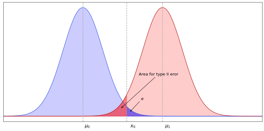
In the plot above the distribution assumed by the null hypothesis has mean value at $\mu_0$ while the true distribution is centered at $\mu_1$. In this case the null hypothesis will not be rejected if the sample mean is greater than $x_0$ (the critical level at significance level $\alpha$). Hence, the probability of type II error will be equal to the area of the true distribution to the left from $x_0$, which can be obtained from the $z$-score at $x_0$ provided that the true mean of the population is $\mu_1$. This probability is usually signed with $\beta$, and the power is then equal to $1-\beta$.
In order to increase statistical power and thus to reduce the probability of type II error we can increase the level of significance so that the overlapping regions are being cut off. This however will make type I error more likely. A better option for increasing statistical power would be to increase the sample size. Since for the normal distribution the values are concentrated around its mean, drawing more samples will have a better chance of getting a sample mean close to the true mean, which is a consequence of the Weak law of large numbers (more to it can be found here). Back to top ↑
Power analysis
Power analysis is a method which helps to define the size of a sample in order to get a certain level of statistical power. It won’t hurt to have a sample of greater size but in practice this might be expensive so the desired minimum should be determined beforehand. Apart from the desired level of statistical power among factors affecting the required sample are the significance level (the smaller the significance level - the larger sample size is needed), type of the alternative hypothesis (whether we have a one- or two-tailed test), the difference between two distributions which needs to be detected, and the variance.
For starters let’s recall the formula for the margin of error when estimating a mean of a population through a sample.
$E = Z \cdot \frac{\sigma}{\sqrt{n}}$
Knowing the population’s standard deviation (or having an estimate of it), the level of significance, and the desired margin of error, it is possible to calculate the required sample size by rearranging the formula:
$n = \frac{Z^2 \sigma^2}{E^2}$
When determining the sample size for the hypothesis test, the significance level, type of the alternative hypothesis, and the detectable difference are selected besides the desired value of statistical power. Let’s look again at the example of overlapping distributions above. If the null hypothesis is incorrect, and the true mean is at $\mu_1$ then we set the desired detectable difference between the initially assumed mean $\mu_0$ and $\mu_1$ as $(\mu_1 - \mu_0)$. If the null hypothesis is true then the margin of error is:
$E_0 = Z_{\alpha} \cdot \frac{\sigma}{\sqrt{n}}$
where $\sigma$ is the estimated standard deviation of the population, and $Z_{\alpha}$ is the critical value for a given significance level. The margin of error $E_0$ here is the distance between $\mu_0$ and $x_0$.
Similarly, if the null hypothesis is false then the margin of error for the distribution with the mean at $\mu_1$ is:
$E_1 = Z_{\beta} \cdot \frac{\sigma}{\sqrt{n}}$
where $Z_{\beta}$ is the probability of type II error, and the margin of error $E_1$ is the distance between $\mu_1$ and $x_0$.
At the same time we have:
$\mu_1 - \mu_0 = E_0 + E_1 = Z_{\alpha} \cdot \frac{\sigma}{\sqrt{n}} + Z_{\beta} \cdot \frac{\sigma}{\sqrt{n}}$
So the formula for the required minimum of the sample size looks like this:
$n = \frac{(Z_{\alpha} + Z_{\beta})^2\sigma^2}{(\mu_1 - \mu_0)^2}$
Multiple hypothesis testing
Sometimes it is impossible to come up with a single metric for performing comparison over two groups. For example a new method of learning is tested across several aspects, such as the ability to keep knowledge in the long-term memory, the intuitiveness of the material, the level of engagement, and the level of stress. Another common case is testing of the effectiveness of some method of treatment against a number of indicators. In these examples there is no compound metric which could be used for a single test. Multiple (or global) hypothesis testing refers to simultaneous testing of multiple hypotheses using the same sample, and checking whether the compound $p$-value exceeds the significance level.
The significance level determines the probability of making type I error, and if there are multiple independent hypotheses, they make up for the total significance level, thus increasing the probability of claiming that the two groups are different (that is making a false discovery). Assuming that the null hypothesis is rejected when at least one of the underlying tests is significant, the family-wise error rate (FWER) can be computed with the following formula:
$\bar \alpha = 1 - (1 - \alpha_i)^n$
where $n$ is the number of hypotheses, and $\alpha_i$ is the significance level of $i$th hypothesis.
It becomes obvious that for a larger number of hypotheses the compound probability of making a false discovery becomes too high. In order to control the family-wise error rate, several approaches have been suggested, among which false discovery rate method (FDR, also known as Benjamini–Hochberg procedure) is one of the most preferred ones, as it helps to keep FWER at an acceptable level while not being too conservative and keeping statistical power. Back to top ↑
Benjamini–Hochberg procedure
The method controls family-wise error rate in multiple testing ensuring that it is less or equal to a given significance level. Before discussing how and why it works let’s note that if the null hypothesis is true then the $p$-values are uniformly distributed between 0 and 1. This concurs with the definition of significance level as the probability of having a small $p$-value (a value between 0 and $\alpha$). If the alternative hypothesis is true then there is a high probability of getting a small $p$-value, so in this case the distribution of $p$-values is highly skewed to the left. To demonstrate this I’ve made a simulation of multiple tests for the scenarios when the null hypothesis is true and false, and visualized the distribution of $p$-values in both cases:
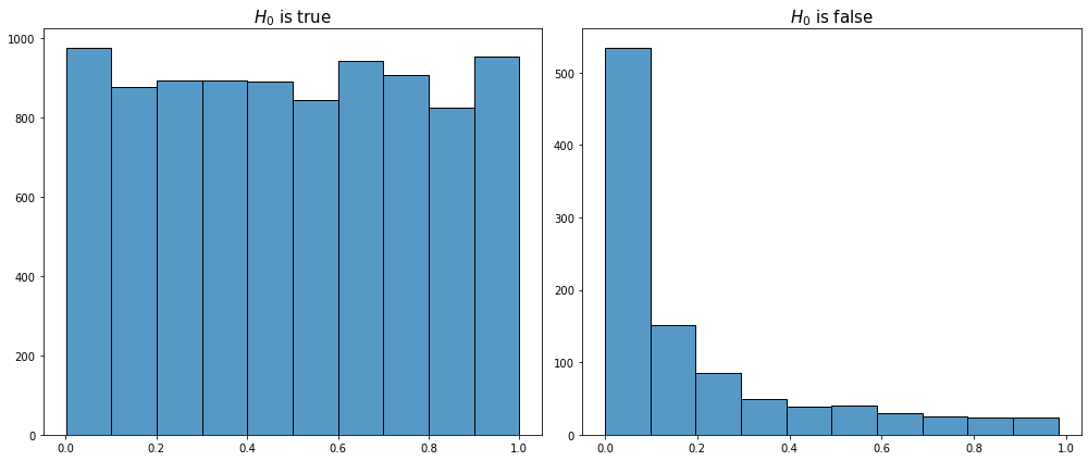
As we see for those samples where the null hypothesis is false we observe a spike at the region of the smallest $p$-values while for the rest of the region the distribution is similar to the uniform. In multiple hypothesis testing we usually have tests for which the null hypothesis is true, and tests for which the null hypothesis is false, so the combined distribution of the $p$-values for the whole global test will look like this (may be viewed as stacking of the charts from above):
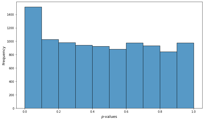
Now, since we want to minimize the number of false positives, we are not going to reject all hypotheses where the $p$-values are less than the significance level. That is we do not reject all hypotheses from the area of the highest column on the histogram of combined $p$-values. Roughly speaking, the idea is in rejecting only $n$ hypotheses from that column, the number of which constitutes the difference between the height of the column and the other columns to the right, since we assume that the lower part of the chart if build from $p$-values of true null hypotheses.
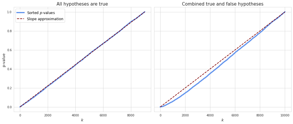
Since the $p$-values are uniformly distributed if the null hypothesis is true, a sorted representation of all $p$-values visually resembles a straight line which can be approximated with the function $\frac{p_k}{n}$, where $p_k$ is the $k$th $p$-value from the sorted row, and $n$ is the number of all hypotheses. If some of the hypotheses are false, as in the case of combined $p$-values, more of them will have small values and thus make the line convex at the beginning.
For the case where not all hypotheses are true it is no longer expected that the function $\frac{p_k}{n}$ approximates the expected $p$-values. Most of the observed values will be smaller than their expectations so the corresponding hypotheses might be all rejected. If all hypotheses are rejected then the rate of false discoveries will be less or equal to 100%:
$\frac{V}{V+S} \leq 1$
where $V$ is the number of incorrectly rejected null hypotheses, and $S$ is the number of correctly rejected ones.
In order to reduce FDR we can simply adjust for a given significance level by transforming $\frac{p_k}{n}$ into $\alpha \frac{p_k}{n}$. Thus FDR will drop and become less than or equal to the significance level $\alpha$.
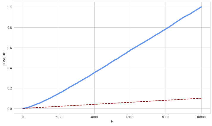
Benjamini–Hochberg procedure basically consists of sorting $p$-values and rejecting only those which are lower than $\alpha \frac{p_k}{n}$. Back to top ↑