Bayesian inference

Bayesian inference is the method of statistical inference where an estimated probability is updated when new data arrives. In a way, it may be viewed as an upgrade of the maximum likelihood estimation(MLE) when some prior knowledge of probability is taken into account.

According to the Bayes’ theorem (or Bayes’ rule) the posterior probability is calculated like this:

     $P(\theta \mid X) = \frac{P(X \mid \theta) P(\theta)}{P(X)}$

Here $\theta$ stands for a hypothesis or a set of parameters according to a particular hypothesis, and $P(\theta)$ is the prior probability which is known before observing the data.
$P(\theta \mid X)$ is the posterior probability of the hypothesis after observing the data $X$.
$P(X \mid \theta)$ is the probability of the data $X$ given the hypothesis $\theta$, in other words, the likelihood function.
$P(X)$ is the probability of observing the data regardless of any hypotheses, also known as the marginal probability.

$P(X)$ is the outcome of all possible joint probabilities $P(X \mid \theta) P(\theta)$ in the space of all possible values of $\theta$. So

     $P(X) = \int_{\theta} P(X \mid \theta) P(\theta) d\theta$

     $P(\theta \mid X) = \frac{P(X \mid \theta) P(\theta)}{\int_{\theta} P(X \mid \theta) P(\theta) d\theta}$

The Bayes’ theorem is derived from the notion of conditional probability. Let’s say we have two events: $A$ and $B$. The conditional probability $P(A\mid B)$ can be intuitively understood as the fraction of probability of event $B$ which intersects with the probability of event $A$: $\frac{P(A\cap B)}{P(B)}$.

Returning to the Bayes’ theorem, both $P(\theta \mid X)$ and $P(X \mid \theta)$ can be expressed in a similar manner using the intersection of probabilities. Then

     $P(\theta \mid X) \cdot P(X) = P(X \mid \theta) \cdot P(\theta)$

     $\frac{P(\theta \cap X)}{P(X)} \cdot P(X) = \frac{P(\theta \cap X)}{P(\theta)} \cdot P(\theta)$

which proves the original formula.

Here is a simple example of the situation where we might want to predict the posterior probability. So let’s suppose that some cafe serviced 287 customers per week, among which 123 left a tip. From the owner’s experience nearly 60% of all customers leave a tip. So how do we factor in the latest observation into the prior knowledge of the probability of leaving the tip?

Below are some of the techniques of Bayesian inference which could be employed.

Bayesian inference is an iterative procedure where the posterior probability is updated each time when new data arrives, and thus it becomes a new prior for the next iteration.

Maximum a posteriori estimation (MAP)

This type of estimation is based on finding the value of $\theta$ where the posterior probability distribution is at its maximum. In the construct of the Bayes’ rule both the prior and the likelihood function depend on $\theta$ while the expression in the denominator does not. This is why maximizing the expression $\frac{P(X \mid \theta) P(\theta)}{P(X)}$ with respect to $\theta$ is the same as maximizing $P(X \mid \theta) P(\theta)$.

$P(X \mid \theta)$ follows the binomial distribution. In our example this is equivalent to the probability of observing the situation where 121 out of 287 customers leave a tip provided that the actual probability of tipping is $\theta$. According to the maximum likelihood estimation, the probability of tipping is nearly 42%.

$P(\theta)$ in turn follows the beta distribution. The choice of this particular distribution is made for convenience because the beta distribution is the conjugate prior of the binomial distribution. It can produce the binomial distribution, and the resulting posterior distribution will also be of the same distribution type. The choice of the parameters $\alpha$ and $\beta$ for the beta distribution here is either subjective or based on some prior statistics like the number successes and failures before carrying out the experiment. For our example let’s pick $\alpha$ as 60 and $\beta$ as 40.

The expression $P(X \mid \theta) P(\theta)$ can be rewritten as product of densities of the two distributions:

     $P(X \mid \theta) P(\theta) = \binom{n}{k} \theta^{k}(1-\theta)^{n-k} \frac{\Gamma(\alpha+\beta)}{\Gamma(\alpha)\Gamma(\beta)} \theta^{\alpha -1}(1-\theta)^{\beta -1} = \binom{n}{k} \frac{\Gamma(\alpha+\beta)}{\Gamma(\alpha)\Gamma(\beta)} \theta^{k+\alpha-1}(1-\theta)^{n-k+\beta-1}$

The point of maximum is obtained by taking the derivative of this expression with respect to $\theta$ and setting it to zero, which further boils down to this:

     $\theta = \frac{k+\alpha-1}{n+\alpha+\beta-2}$

In our example the updated value of the probability of tipping becomes (123+60-1)/(287+60+40-2) which is approximately 47%. Let’s also see how all three probabilities are distributed on the scale from 0 to 1.

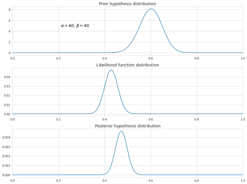
As we can see, the existence of the prior hypothesis slightly shifted the distribution resulting from the MLE towards bigger values. In addition, its values are less spread around its mean because now the distribution incorporates more data.

Note that the choice of $\alpha$ and $\beta$ may significantly impact the posterior distribution. Greater values means higher confidence in the prior hypothesis, so that it has more weight in determining the posterior.

Also note that since we have omitted dividing by $P(X)$ in the calculation of the posterior distribution the function above is not scaled, so it’s not quite the same as the probability density function.

Expected a posteriori estimation (EAP)

This is yet another method of Bayesian inference which is based on the mean of the posterior distribution instead of its mode as is the case with the MAP. Since the posterior is beta-distributed, it is not symmetric, and the mean is usually not equal to the mode.

The mean is calculated through integration over $\theta$ for each possible value of $\theta$ multiplied by its probability density function.

     $E[P(\theta \mid X)] = \int_{\theta} \theta P(\theta \mid X) d\theta = \frac{k+\alpha}{n+\alpha+\beta}$