Probability Distributions
A probability distribution is a function that describes the likelihood of a random variable taking on certain values. Think of it as a model or blueprint for a dataset, showing us the probable outcomes of a random process.
By identifying the distribution that best fits our data, we unlock powerful insights, make informed predictions, and choose the right statistical tests for our analysis.
Discrete vs. Continuous Distributions
Probability distributions are broadly categorized based on the type of data they model.
Discrete Distributions: These deal with variables that have a finite or countable number of outcomes. The distribution is described by a Probability Mass Function (PMF), which assigns a specific probability value to each individual outcome. For example, the number of heads in a series of coin tosses.
Continuous Distributions: These are for variables that can take any value within a given range. The distribution is described by a Probability Density Function (PDF), which gives the relative likelihood of a variable taking a certain value. While the probability of a continuous variable assuming an exact value is zero, the PDF allows us to calculate the probability of the variable falling within a specific range using integral calculus.
Common Discrete Distributions
These distributions are used to model count data and other discrete random variables.
Bernoulli Distribution
This is the simplest of all distributions, representing a single trial with two outcomes (e.g., 0 or 1). It’s essentially a binomial distribution with a single trial ($n$=1). It models events like a single coin flip.
Binomial Distribution
The binomial distribution is a discrete probability distribution that models the number of “successes” in a fixed number of independent experiments, where each experiment has only two possible outcomes. These individual experiments are known as Bernoulli trials. A classic example is a coin toss, where the outcome is either heads or tails. However, any experiment can be considered a Bernoulli trial by defining one outcome as a “success” and all others as a “failure.” For a continuous variable, a Bernoulli trial can be created by setting a threshold and considering “crossing the threshold” as a success and “not crossing it” as a failure.
A random variable follows a binomial distribution if it represents the number of successes in a sequence of independent Bernoulli experiments. The probability mass function (PMF) is constructed using the knowledge of the probability of success in a single experiment:
\[f(x) = {\binom{n}{x}}p^{x}(1-p)^{n-x}\]where $p$ is a probability of success in a single experiment, $x$ is the number of expected successes, $n$ is the number or experiments, and where $\binom{n}{x}$ is the binomial coefficient, which represents the number of ways to choose $x$ successes from $n$ experiments:
\[\binom{n}{x} = \frac{n!}{x!(n-x)!}\]Assumptions and Key Parameters of the Binomial Distribution
The binomial distribution relies on a few key assumptions:
- The experiments are independent of each other.
- The probability of success ($p$) remains the same for each individual trial.
- The number of trials ($n$) is fixed.
As we can see from the formula, the two main parameters defining a binomial distribution are n (the number of trials) and p (the probability of success).
Mean and Variance of the Binomial Distribution
We can determine the expected value (mean) and variance of the binomial distribution from the properties of a single Bernoulli trial. Let’s assign a value of 1 to a successful outcome and 0 to a failure. The expected value (or mean) for a single trial is then:
\[E(x) = 1 \cdot p+0 \cdot (1-q) = p\]From this, the expected value (or the mean) of the entire binomial distribution is simply the sum of the expected values of all trials, which is $np$.
The variance measures the sum of squared distances between the observed and expected values. For a single Bernoulli trial, the variance is calculated as:
\[\begin{align*} \text{Var}(x) &= p(1-p)^2+(1-p)(0-p)^2\\ &= p(1-p)^2+(1-p)p^2\\ &= p(1-p)(1-p+p)\\ &= p(1-p) \end{align*}\]Therefore, the variance for the binomial distribution is $np(1-p)$.
The Normal Approximation
In order to achieve better accuracy with binomial distribution testing the whole experiment may be performed multiple times (or the observations may be resampled with replacement). For example we want to estimate how well the audience likes a new movie. The outcome for each individual cinema visitor is viewed as a Bernoulli trial while the number of satisfied visitors after a session is the result of a single binomial test. Since this measure itself may depend on many factors the results after each session may be quite different. In order to understand the average percentage of the audience satisfaction it may be useful to visualize with a histogram the total number of outcomes for the binomial tests across all sessions. Below is a plot displaying distribution of binomial test results for 1000 sessions each containing 200 visitors.
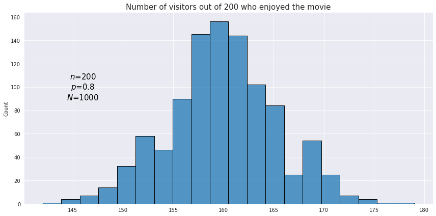
If the number of experiments is reasonably high (specifically, if both $np$ and $n(1−p)$ are greater than 5), the binomial distribution may be closely approximated by the normal distribution. As shown in the image above, the resulting values of a binomial experiment will be concentrated around a certain central value, demonstrating a behavior similar to that of a normal distribution.
Poisson Distribution
This distribution is used to model the number of events which occur during a fixed period of time, for example the number of customer complaints per month or the number of trains arriving during a certain hour. Similarly to the binomial distribution, all occurrences of events are considered random and independent, so the occurrence of one event does not affect the probability of another event.
The probability mass function of the Poisson distribution uses prior knowledge of the average number of occurrences per period - parameter $\lambda$. This parameter can actually be derived from the binomial distribution as $\lambda = np$, where $p$ is the probability of a single event occurrence, and $n$ is the number of Bernoulli trials. Both mean and variance of a random variable which follows the Poisson distribution are equal to $\lambda$, and this is the formula of its PMF:
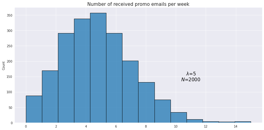
\[f(x; \lambda) = \frac{\lambda^{x}e^{-\lambda}}{x!}\]For example, a person receives on average 5 promotional emails from different sellers. The probability of receiving 3 emails would be
\[f(3; 5) = \frac{5^{3}e^{-5}}{3!} \approx 0.14\]Here is an example of an observed distribution of the number of received emails for a sample of 2000 users.
Geometric distribution
This is a type of distribution which is used to model the number of failures in sequences of Bernoulli trials before the first success (or vice versa). For example we want to know how many customers a retail shop has to engage with before the first sale is made.
The PMF of the geometric distribution is given by the following formula:
\[f(x) = (1-p)^{x} p\]The formula is pretty intuitive as it just calculates the joint probability of $x$ failures in Bernoulli trials, each having probability of $(1-p)$, and 1 success probability of which is $p$.
Below is an example of what an observed geometric distribution could look like:
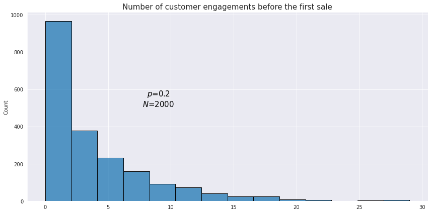
From our example above the probability of having the first successful sale after 2 unsuccessful customer engagements would be
\[f(2) = (1-0.2)^{2} \cdot 0.2 = 0.128\]The mean of the geometric distribution is defined as $\frac{1-p}{p}$.
Negative binomial distribution
This distribution is the generalization of the geometric distribution which is used to model the number of failures before the $n$th success. The PMF is the following:
\[f(x; r) = \binom{x+r-1}{r-1}(1-p)^{x}p^r\]where $r$ is the required number of successes, $p$ is the probability of a success in a single Bernoulli experiment.
Using the same example as with the geometric distribution, let’s see how the distribution looks like for the number of unsuccessful customer engagements before 10 sales were made.
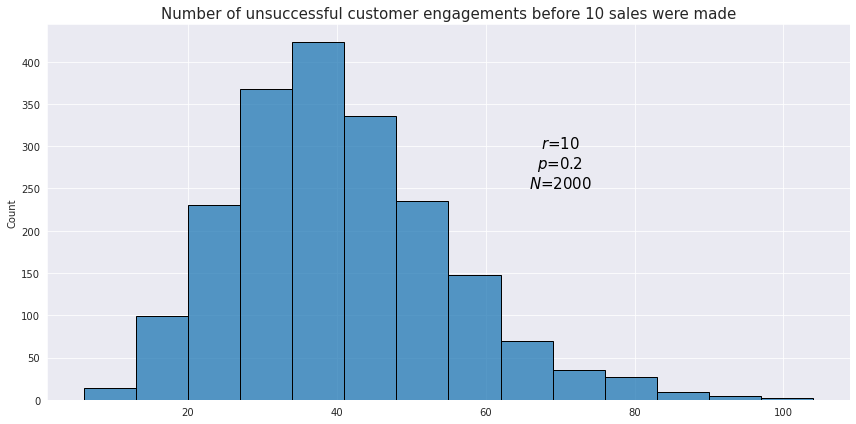
The mean of the negative binomial distribution is defined as $\frac{r(1-p)}{p}$, and the variance is $\frac{r(1-p)}{p^2}$.
Negative Binomial as Generalization over Poisson Distribution
The negative binomial distribution is, in fact, often used as a generalization of the Poisson distribution to handle a specific and common issue in count data called overdispersion. Overdispersion occurs when the variance of the data is greater than its mean.
The Poisson distribution makes a strong assumption: its mean is equal to its variance. This works well if events are truly random and independent. However, in real-world data like the number of crashes per device device, the variance is often larger than the mean. This might happen if certain factors (like a specific software bug, heavy usage, or a particular device model) cause some devices to be much more prone to crashing than others. This “extra” variability is not accounted for by the Poisson model.
The negative binomial distribution addresses this by including an extra parameter $\alpha$ that allows the variance to be greater than the mean. It is a more flexible model that can capture this additional, unobserved variability. In order to do that the parametrization of the distribution model needs to shift from $r$ and $p$ to more intuitive $\mu$ and $\sigma$.
In an alternative parametrization model the mean represents the average number of events (e.g., crashes per hour).
The variance is given by:
\[\sigma=\mu + \alpha \mu^2\]where $\alpha$ is a dispersion parameter that quantifies the overdispersion. When $\alpha$ approaches zero, the negative binomial distribution’s variance approaches its mean, and its shape converges to that of a Poisson distribution.
Derivation of the Alternative Negative Binomial Distribution Parametrization
Using the definition of the mean:
\[\frac{1-p}{p} = \frac{\mu}{r}\]Then putting this into the variance formula:
\[\sigma^2 = \frac{r(1-p)}{p^2} = \frac{r(1-p)}{p} \times \frac{1}{p} = \mu \times \frac{1}{p}\]This gives us the variance in terms of the mean and the probability of success. Now, let’s use the first equation again to express $p$ in terms of $\mu$ and $r$:
\[1- p = \frac{\mu p}{r}\] \[1 = p + \frac{\mu p}{r} = p(1+\frac{\mu}{r})\] \[p = \frac{1}{1+\frac{\mu}{r}}\]Finally, substitute this expression for p back into the variance formula:
\[\sigma^2 = \mu \times (1+ \frac{\mu}{r}) = \mu + \frac{\mu^2}{r}\]So $\alpha$ is actually $\frac{1}{r}$.
Uniform Distribution
This type of distribution describes processes where every possible outcome has the same chance of occurring. It could be either discrete of continuous. An example of a discrete uniform distribution is rolling of a dice once and expecting any of the possible 6 values.
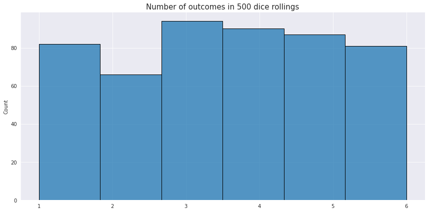
The PMF for the discrete distribution is just $\frac{1}{n}$, where $n$ is the number of partitions with the equal probability.
For the continuous distributions the PDF is a constant line:
\[f(x) = \frac{1}{b-a}\]where $a$ and $b$ are the borders of the distribution.
The expected value of the uniform distribution is defined as the center of the range over which the value is distributed $\frac{a+b}{2}$.
Common Continuous Distributions
Normal Distribution
Normal distribution, also known as the Gaussian distribution, is arguably the most important and widely used distribution in statistics. It is characterized by its symmetric, bell-shaped curve. Many natural phenomena follow this pattern, such as the height of people, blood pressure, and test scores. The normal distribution is completely defined by its mean ($\mu$) and standard deviation ($\sigma$). Since this is a foundational distibution, it has its own dedicated page.
Student’s t-Distribution
The Student’s t-distribution is a continuous probability distribution that is very similar in shape to the normal distribution. However, it is specifically designed for situations where the sample size is small and the population standard deviation is unknown. Its most distinguishing feature is its fatter tails, which account for the greater uncertainty that comes from working with a small sample of data.
Unlike the normal distribution, which has a constant shape, the shape of the t-distribution changes based on a single parameter: the degrees of freedom ($\nu$).
Properties of Student’s t-Distribution
-
Degrees of Freedom ($\nu$): This parameter is directly related to the sample size ($n$). The degrees of freedom are calculated as $n$−1.
-
Fatter Tails: The “fatter tails” mean that the t-distribution assigns a higher probability to extreme values compared to the normal distribution. This reflects the reality that with a small sample, you are more likely to encounter an extreme value by chance.
The key property of this distribution is its relationship with the normal distribution. As the degrees of freedom increase (i.e., as the sample size grows), the t-distribution’s shape becomes virtually identical to the standard normal distribution.
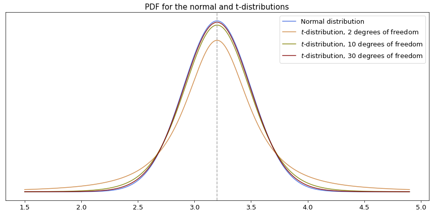
As the size of the sample (and therefore the degrees of freedom) increases, the t-distribution becomes virtually identical to the normal distribution. For a sample size of roughly 30 or more, the two distributions are so close that they can be used interchangeably.
Why Is Student’s t-Distribution So Important?
The t-distribution is a cornerstone of inferential statistics because it provides a reliable method for analyzing data from small samples.
Its primary use is in:
-
Hypothesis Testing: It is used in the t-test to determine if the means of two groups are significantly different from each other when the sample size is small and the population variance is unknown.
-
Confidence Intervals: It is used to construct confidence intervals for a population mean using inferential statistics. This allows us to estimate a range of plausible values for the true population mean based on a small sample.
In essence, while the normal distribution is the “ideal” model for a large population, the t-distribution is the practical and more robust tool for when we have limited data.
Similar to how z-scores and z-tables are used for the normal distribution, the t-distribution has its own tables of precomputed values for different levels of degrees of freedom. This is incredibly useful for practical applications, as it means there is no need to perform complex integration over its probability density function when calculating probabilities.
Chi-squared distribution
In a nutshell the chi-square distribution is the distribution of sum of squared values sampled from a normally distributed variable.
\[\chi_k^{2} = \sum_{i=1}^k Z_i^2\]where $Z_i$ is a randomly drawn value from a normal distribution, and $k$ is the number of degrees of freedom, which is also equal to the number of drawn values.
Below is a visualization of the probability density function of the chi-square distribution for a different number of degrees of freedom if the values are drawn from the normal distribution with the mean value 0, and the standard deviation 1.
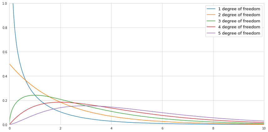
Notice that since we are squaring the values there are no negative values in the chi-square distribution. If we draw only one value, then there is a high probability that this value is close to 0, since the normal distribution is centered around 0. Therefore the shape of the PDF of chi-square distribution with 1 degree of freedom is heavily skewed towards zero, while the probability of getting bigger numbers becomes minuscule. If we draw more and more numbers increasing the number of degrees of freedom, the sum of squared values causes the center of the PDF of chi-square distribution to be shifted to the right.
Beta Distribution
This distribution is an extension of the negative binomial distribution to the continuous variables. However, instead of modeling the number of successes (or failures), it is used for modeling the distribution of probability.
Let’s imagine that out of 100 customers who went to a gym trial, only 63 decided to buy an annual membership. How would one describe the probability of purchasing a gym membership after trying a trial? The most obvious answer would be say 63%, and this is not wrong, yet it might be useful to resort to a distribution instead of picking just one number for probability. See, 63% is the statistic of a sample, and the true percentage might be different. As such, we might want to know the probability that the true probability of buying a gym membership is greater than 50% for example. This is where the beta distribution comes to rescue because using its probability density function we can simply integrate over all its values higher than 0.5.
The beta distribution is defined for the inclusive range between 0 and 1, and its PDF looks like this:
\[f(x; \alpha, \beta) = \frac{x^{\alpha -1}(1-x)^{\beta -1}}{\mathrm{B}(\alpha, \beta)}\]where $\alpha$ and $\beta$ reflect the proportion of successes and failures accordingly, and $\mathrm{B}(\alpha, \beta)$ is a normalization coefficient defined as follows:
\[\mathrm{B}(\alpha, \beta) = \frac{\Gamma(\alpha)\Gamma(\beta)}{\Gamma(\alpha+\beta)}\]The gamma-function $\Gamma$ is an extension of the factorial expression to complex numbers which makes it possible to use it for a continuous range of numbers.
\[\Gamma (n) = (n-1)! = \int_{0}^{\infty} x^{n-1}e^{-x} dx \text{ for } n > 0\]Now, when we look at the formula of the PDF of the distribution more closely, we can see that it is very similar to the PMF of the negative binomial distribution. Since the beta distribution is continuous, the binomial coefficient from the binomial distribution is replaced with the expression which consists of the gamma functions:
\[\binom {n}{k} = \frac {n!}{k!(n-k)!} = \frac{\Gamma(n+1)}{\Gamma(k+1)\Gamma(n-k+1)} = \frac{1}{\mathrm{B}(k+1, n-k+1)}\]Below we can see how the probability density function of the beta distribution would look like depending on the choice of the parameters.
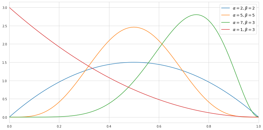
It is worth mentioning that the higher the value of the parameters - the tighter the values are centered around its mean, which reflects the certainty about the distribution.
The mean of the beta distribution is defined as $\frac{\alpha}{(\alpha+\beta)}$, and the variance is $\frac{\alpha\beta}{(\alpha+\beta)^2(\alpha+\beta+1)}$.
Exponential Distribution
This is a continuous distribution which is closely related to the Poisson distribution as it models the time between random independent events. It may also be viewed as a continuous analogue of the geometric distribution. The PDF of the distribution is calculated as follows:
\[f(x; \lambda) = \lambda e^{-\lambda x}\]Suppose we would like to model the time between arrival of two buses at some station when on average there are 4 incoming buses for an hour. Translating this into minutes we have $\lambda = \frac{4}{60} \approx 0.07$. This is what a hypothetical distribution of time in minutes would look like:
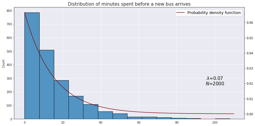
The mean of the exponential distribution is $\frac{1}{\lambda}$, and the variance is $\frac{1}{\lambda^2}$.
Weibull Distribution
This distribution is a cornerstone of survival analysis, specifically within the framework of parametric survival models.
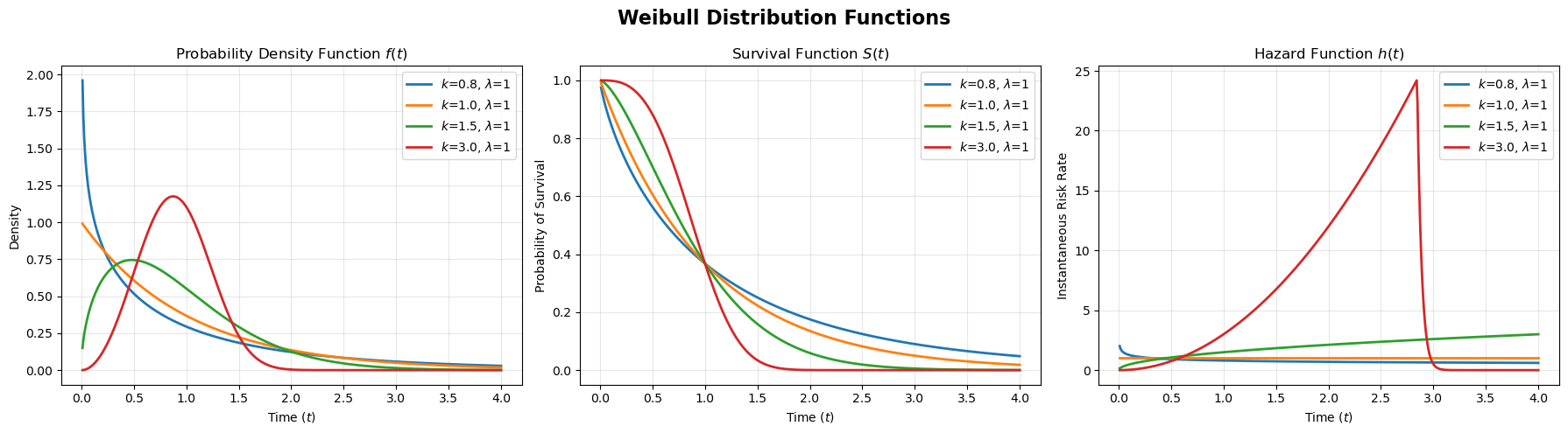
While the Exponential distribution assumes a constant rate of events (constant hazard, in survival analysis terminology), the Weibull distribution relaxes this assumption by adding a parameter that allows the risk to change over time. This flexibility better reflects the real world, where organisms age, machines wear out, and biological systems adapt.
The Shape Parameter $k$ dictates the behavior of the hazard.
- $k<1$ (Decreasing Hazard): The risk is high at the start and drops over time. For example in post-surgery survival the highest risk is immediately after the operation: if you survive the first week, your chances of long-term survival improve significantly.
- $k=1$ (Constant Hazard): The risk never changes. In this case the Weibull distribution mathematically transforms into the Exponential distribution.
- $k>1$ (Increasing Hazard): The risk starts low and grows over time. For example a car tire works fine when new, but as miles accumulate, the probability of a blowout increases.
The Scale Parameter $\lambda$ stretches or shrinks the curve along the time axis, affecting the time scale of the event (e.g., days vs. years).
The probability density function (PDF) is given by:
\[f(t) = \frac{k}{\lambda}\left(\frac{t}{\lambda}\right)^{k-1}e^{-(t/\lambda)^k}\]We can better understand this equation by viewing it through the lens of the fundamental survival relationship, where the density is the product of the hazard and the survival function, $f(t) = h(t) S(t)$.
-
The term $e^{-(t/\lambda)^k}$ is the survival function $S(t)$. As $t$ increases, this term decays to 0, representing the probability of survival decreasing over time.
-
The term $\frac{k}{\lambda}\left(\frac{t}{\lambda}\right)^{k-1}$ is the hazard function $h(t)$. This term controls the “instantaneous risk”. For example, if $k=2$ the hazard grows linearly with time, and if $k=1$ the hazard becomes constant.
Log-Normal Distribution
This distribution arises when the logarithm of a random variable is normally distributed.
\[X = e^{\mu + \sigma Z}\]While the normal distribution results from adding independent random events (the additive Central Limit Theorem), the log-normal distribution results from the multiplication of many independent random effects.
Similar to the normal distribution, the parameters of the log-normal distribution are $\mu$ and $\sigma$, but they refer to the underlying logged data:
-
$\mu$ is the mean of the logged data ($\ln T$). It functions as a scale parameter: if $\mu$ increases, the entire curve shifts to the right.
-
$\sigma$ is the standard deviation of the logged data. This parameter controls the shape (skewness). A higher $\sigma$ results in a much heavier, longer tail to the right, indicating a higher probability of extreme outliers.
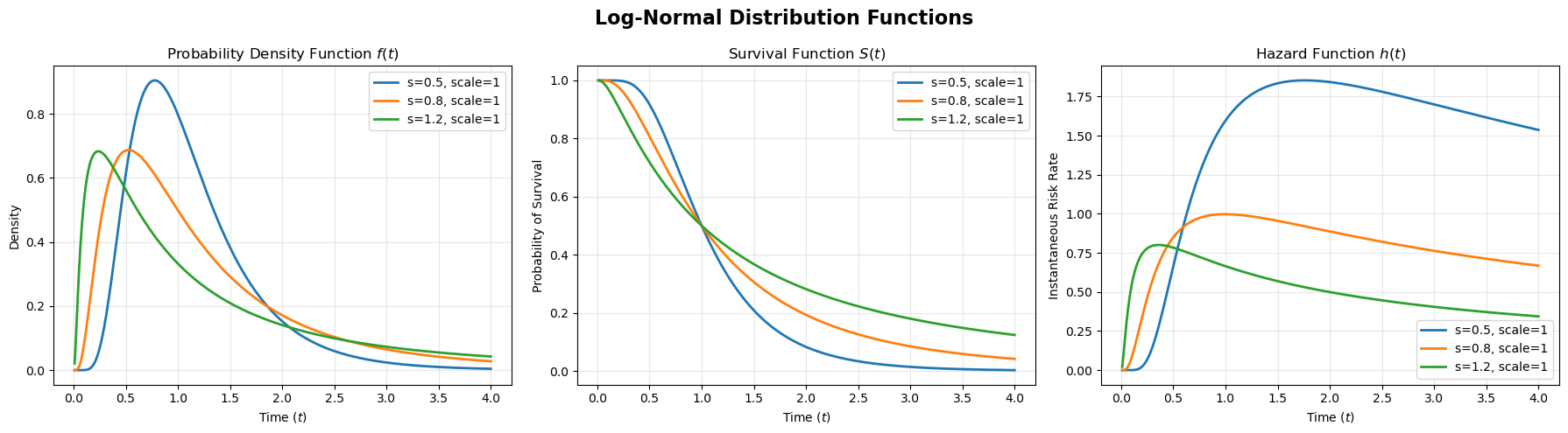
This distribution is used in survival analysis to model the hazard rate which increases in time up to a certain point, and then becomes smaller. For example the risk of dying immediately after a surgery is small, but then rises quickly to a peak (complications usually happen here), and if you survive that peak, your risk drops the longer you live.
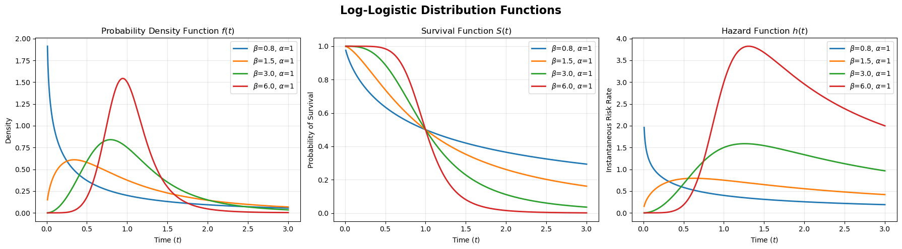
Log-Logistic Distribution
The Log-Logistic distribution is the “cousin” of the Log-Normal. To the naked eye, their density plots look almost identical (both are right-skewed humps), but the Log-Logistic has heavier tails (more outliers).
Mathematically, it is the distribution of a variable $T$ whose logarithm follows a Logistic distribution. The Standard Logistic distribution is very similar to the standard normal distribution, but, again, with heavier tails.
Recall the cumulative distribution function (CDF) of a standard logistic variable $z$ (from logistic regression):
\[F(t) = \frac{1}{1+e^{-t}}\]The derivative gives the probability density function:
\[f(t) = \frac{e^{-t}}{(1+e^{-t})^2}\]We can define $Y= \ln(T)$ which follows a logistic distribution with location parameter $\mu$ (often mapped to $\ln(\alpha)$) and scale parameter $s$ (often mapped to $1/\beta$). Solving it for $T$ creates as log-logistic distribution, and this is how its PDF looks like when parametrized via $\alpha$ and $\beta$:
\[f(t) = \frac{(\beta/\alpha)(t/\alpha)^{\beta-1}}{(1+(t/\alpha)^\beta)^2}\]In the context of survival analysis, we can break this down into the survival function and the hazard function:
\[S(t)=\frac{1}{1+(t/\alpha)^\beta}\] \[h(t)=\frac{(\beta/\alpha)(t/\alpha)^{\beta-1}}{1+(t/\alpha)^\beta}\]The numerator of the hazard function resembles the Weibull hazard. It pulls the risk up (if $\beta>1$). However, the denominator ($1+(t/\alpha)^\beta$) grows faster than the numerator as $t$ gets very large. This forces the hazard to eventually turn around and decrease, creating a “hump” shape similar to the Log-Normal distribution.