Normal Distribution

Introduction

Normal distribution (also known as Gaussian distribution) is one of the most fundamental building blocks of Probability and Statistics. It serves as a cornerstone for statistical inference and is used to model a vast range of phenomena in the natural and social sciences. Its distinctive, symmetric shape is what makes it so recognizable and powerful.

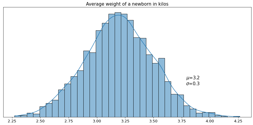
Suppose, we decided to measure the weight of all newborns in a multitude of different hospitals and calculate the average weight in each hospital. Most likely the distribution of those average weights will resemble a bell-shaped curve.

Here we see that the average of all measured averages converges around a certain central value, 3.2 kilos in this case. This means that among all measured averages we encountered mostly values which are very close or equal to 3.2. The closer the hospital average to 3.2 - the higher the frequency of such encounters. By contrast, we see that there are very few averages that have values, say, higher than 4 or lower than 2.5 kilos. The bell-shaped function that we have above is actually the approximation of probability density function for the given distribution, and its values provide relative likelihood of a random variable (in our example the weight of the newborn) to assume certain values.

Properties and Function Defintion

The normal distribution is defined entirely by two parameters:

• Mean ($\mu$): This is the average of the data and represents the center of the distribution. It’s the point where the bell curve is at its peak.

• Standard Deviation ($\sigma$): This measures the spread or dispersion of the data. A small standard deviation indicates that the data points are tightly clustered around the mean, resulting in a tall, narrow curve. A large standard deviation means the data is more spread out, creating a flatter, wider curve.

Probability Density Function of Normal Distribution

The formula for the probability density function (PDF) of the normal distribution, often called the Gaussian function. It provides the mathematical blueprint for the bell-shaped curveand

\[f(x) = \frac{1}{\sigma\sqrt{2\pi}}e^{-\frac{1}{2}(\frac{x-\mu}{\sigma})^2}\]

Notice the expression $\frac{x-\mu}{\sigma}$. This is a z-score, and it measures how many standard deviations a specific value, x, is from the mean. We’ll use this crucial expression later for calculating probabilities and performing hypothesis testing. For now, just think of it as a standardized measure of distance from the mean.

The Probability Density Function (PDF) for the normal distribution is an exponential function. The exponent is negative and squared, which is what creates the characteristic bell shape. The negative sign ensures the function decreases as you move away from the center, preventing it from “skyrocketing.” Squaring the term $\frac{x-\mu}{\sigma}$ makes the function symmetric around the mean, as both positive and negative distances from the mean will result in a positive squared value, leading to the same height on the curve. This is why the curve drops off equally on both sides.

The inclusion of the mean ($\mu$) and standard deviation ($\sigma$) in the exponent ensures the function is centered at its mean, not zero, and has the correct spread (narrow or wide) that matches the data.

The division by 2 in the exponent and the scaling factor $\frac{1}{\sigma\sqrt{2\pi}}$ are both essential for a single purpose: to ensure that the total area under the curve is exactly 1. This is a fundamental property of all probability density functions, as the total probability of all possible outcomes must equal 100%. These terms mathematically “normalize” the function, so it properly represents a probability distribution.

Why Is It So Important?

The normal distribution’s significance stems from two key reasons: its prevalence in the real world and a crucial mathematical principle.

Firstly, many naturally occurring variables follow a normal or near-normal distribution. Examples include human height, blood pressure, IQ scores, and measurement errors in scientific experiments. This makes it a valuable model for understanding and predicting these variables.

Secondly, and most importantly, is the Central Limit Theorem (CLT). This theorem states that the distribution of sample means will approximate a normal distribution, regardless of the population’s underlying distribution, as long as the sample size is sufficiently large. This remarkable property allows us to use the normal distribution to make inferences about a population from a sample, which is the very foundation of inferential statistics.

Using the Normal Distribution

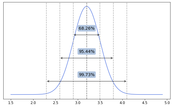
Because its properties are well-understood, we can use the normal distribution to calculate probabilities, such as the likelihood that a random variable will fall within a certain range. A common rule of thumb for the normal distribution is the 68-95-99.7 rule (or six sigma rule), which states that approximately:

• 68% of the data falls within one standard deviation of the mean.
• 95% of the data falls within two standard deviations of the mean.
• 99.7% of the data falls within three standard deviations of the mean.

This rule provides a quick way to understand the spread of data and identify potential outliers. In practice, the normal distribution is an essential tool for hypothesis testing, confidence intervals, and predictive modeling, making it an indispensable concept for anyone working with data.

Based on the example above, we may deduce that:

• 68.26% of all newborns have weight from 2.9 to 3.5 kilos (one standard deviation away from the mean)
• 95.44% - from 2.6 to 3.8 kilos (two standard deviations away from the mean)
• 99.73% - from 2.3 to 4.1 kilos (three standard deviations away from the mean)

Probability of Getting Certain Interval values

Before moving on, let’s re-introduce the z-score metric. Plainly speaking, $z$-score tells us how many standard deviations a given value is away from the mean of its distribution.

     $z = \frac{x-\mu}{\sigma}$

In general, in order to calculate the area under the curve we would have to perform integral calculus. Integrating over the PDF produces the the cumulative distribution function (CDF). However, for the normal distribution, we can use a z-table to find probabilities without having to do any complex math.

A z-table is a precalculated table of values from the cumulative distribution function (CDF) of the standard normal distribution. It shows the probability of a random variable taking on a value less than a specific z-score.

There are two main types of z-tables: those that show the area to the left of the z-score and those that show the area between the z-score and the mean. While the most common z-tables cover both positive and negative z-scores, they are often presented in separate parts for scores that are above the mean (positive) or below the mean (negative). This allows for easy look-up of probabilities for values on either side of the distribution’s center.

Suppose we want to calculate the percentage of newborns who have weight less than 3 kilos and the percentage of newborns with weight from 3 to 3.5 kilos. That is equal to calculating the filled areas under the curves below.

In the first case we simply calculate $z$-score of the value 3 and look up the area under the curve from the $z$-table for negative values (since 3 is lower than the mean 3.2). In this example it approximates to 0.2514. So conclude that only 25.14% of all newborns have weight 3 kilos or less.

In the second example we have an area with two cut-off points. $Z$-table allows us to find the area to the left from a specific value, so here is what we do. First we calculated $z$-scores for 3.5 and for 3, then we looked up the area under the curve for all weights which are less than 3.5 kilos and those which are less than 3 kilos. Then we simply subtract the second from the first. Finally we end up with something like 0.8413 - 0.2514, which equals 0.59. Here we conclude that nearly 59% of all newborns have weight between 3 and 3.5 kilos.