Descriptive Statistics

Introduction

Descriptive Statistics is the essential first step in any data analysis, providing the tools to summarize, organize, and present data in a clear, understandable way. Unlike inferential statistics, which makes predictions, descriptive statistics simply describes the data available, revealing its key patterns and characteristics.

Descriptive statistics relies on the following categories:

• Measures of Central Tendency: Where the data values tend to cluster or center.
• Measures of Variability: How spread out or dispersed the data is.
• Measures of Distribution Shape: The overall form of the data’s distribution when visualized.

Measures of Central Tendency

These measures provide a single value that represents the center of a dataset.

The Mean (Average): The most common measure. It is calculated by summing all values and dividing by the number of values.

\[\overline x = \frac{\sum x}{n}​\]

It is easily affected by extreme values or outliers.

The Median: The middle value of an ordered dataset. If a dataset has an even number of data points, it is the average of the two middle values.

It is a robust measure that is not sensitive to outliers.

The Mode: The value that appears most frequently in a dataset.

This is particularly useful for categorical data.

Choosing between the Mean and and Median

Even though median better represents the typical observation value and is robust against the outliers there is a a number of reasons to use mean in statistical applications:

The mean is algebraically simple and has nice mathematical properties. It can be easily manipulated in equations, which is why it appears naturally in formulas for variance, standard deviation, correlation, regression, and many other statistical tools. At the same time the median, while robust, is harder to use in closed-form calculations.

The mean uses all data points in its calculation, not just the middle one. This makes it more sensitive to variation in the data, which is often what analysts want. The median only depends on order, so it ignores actual magnitudes beyond rank.

When we sample repeatedly then according to the Central Limit Theorem, the distribution of the sample mean approaches a normal distribution (even if the original data is not normal). This makes the mean extremely useful for inference, confidence intervals, and hypothesis testing. The median doesn’t share this property in the same way.

Measures of Variability (Dispersion)

Central tendency describes the center, while these measures describe how much the data values vary from each other.

The Range: The simplest measure, calculated as the difference between the highest and lowest values. It is quick but limited as it only uses two data points.

The Variance: The average of the squared differences from the mean.

\[\sigma^2=\frac{\sum (x−μ)^{2}}{N}\]

The units are squared, which can make it hard to interpret.

The Standard Deviation: The square root of the variance. It is the most common measure of dispersion because it is in the same units as the original data.

\(\sigma=\sqrt{\frac{\sum (x−μ)^{2}}{N}}\) ​ The Interquartile Range (IQR): The range of the middle 50% of the data. It is the difference between the first and third quartiles (Q3​−Q1​) and is not affected by outliers.

Describing the Distribution Shape

The shape of the data distribution can reveal important insights.

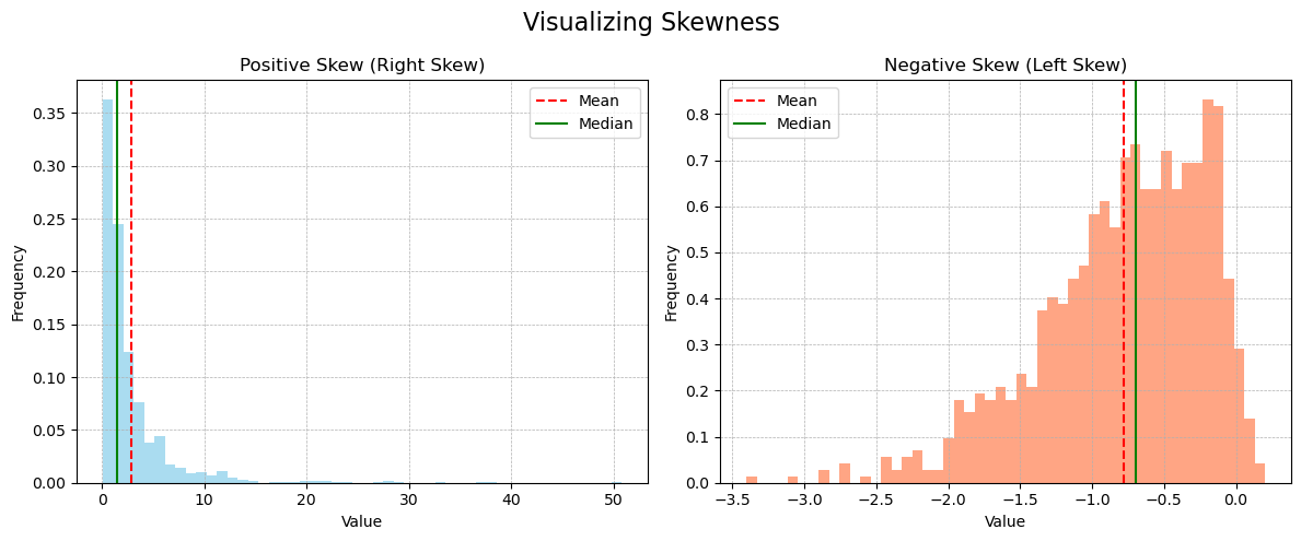
Skewness: A measure of the asymmetry of a distribution. Positive skew means he tail on the right side is longer or fatter, and vice versa.

Kurtosis: A measure of the “tailedness” of a distribution.

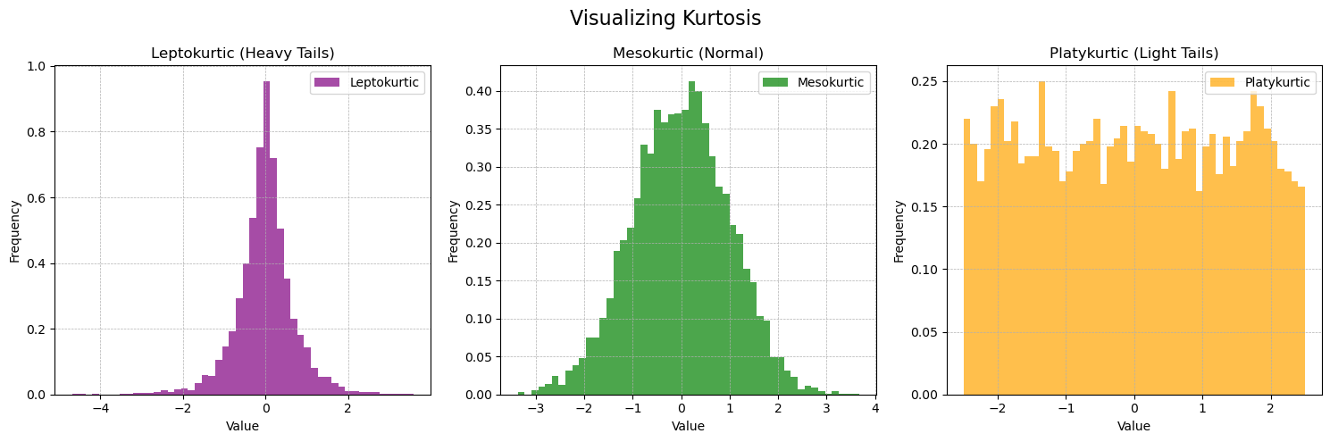
Here Leptokurtic distribution means having sharper peaks and more extreme value leading to heavier tails. Platykurtic on the other hand are flatter indicating fewer extreme value.

Visualizing Descriptive Statistics

• The Histogram: Displays the frequency of data within different ranges.
• The Box Plot: A five-number summary showing the median, quartiles, and outliers.
• The Scatter Plot: Used to visualize the relationship between two variables.