Bootstrapping

Introduction

In traditional statistics, we rely on a theoretical framework—like the Central Limit Theorem to determine the sampling distribution of a statistic. But what happens when our data doesn’t fit the assumptions of these theorems, or when we are interested in a statistic (like the median or a 90th percentile) for which there is no simple formula for its standard error?

This is where bootstrapping comes in. Bootstrapping is a modern, computer-intensive method that allows us to simulate a sampling distribution from our single, existing sample. It is a powerful technique that helps us to estimate a statistic and, most importantly, quantify the uncertainty around that estimate.

The Core Idea: Resampling with Replacement

Imagine we have a single sample of data, perhaps 20 values representing the monthly sales of a product. We want to estimate the median sales and build a confidence interval around it. Instead of relying on a theoretical formula, bootstrapping uses the data we already have to create thousands of new “bootstrap” samples.

The process works like this:

1. Take one sample: we start with your original sample of data.
2. Resample: we take a new sample of the same size as your original sample, but we do it with replacement. This means that a value is randomly selected from our original sample, gets recorded, and then put back. We repeat this process until our new “bootstrap” sample is the same size as the original. Because we are sampling with replacement, some values from the original sample will appear multiple times in the new sample, while others may not appear at all.
3. Calculate the statistic: we compute the statistic of interest (e.g., the median) for this new bootstrap sample.
4. This is repeated many times (e.g., 5,000 to 10,000 times) to create a large collection of bootstrap statistics.

Why Bootstrapping is so Useful

After running the bootstrapping process, we are left with a collection of thousands of sample medians. This collection of values is a simulated sampling distribution. We have effectively created the “map” that we discussed in our article on sampling distributions, but we did it without needing to take a new sample or rely on a theoretical formula.

From this simulated distribution, we can:

• Estimate the standard error: The standard deviation of your bootstrap medians is the standard error of the median.
• Construct a confidence interval: A simple way to do this is to take the 2.5th and 97.5th percentiles of our simulated sampling distribution. This gives us a 95% confidence interval for the population median.
• Visualize uncertainty: By plotting the histogram of your bootstrap statistics, we can see the shape and spread of your sampling distribution, giving a clear visual sense of the uncertainty.

Below is an example of such calculation of a confidence interval for the median of hypothetically skewed data.

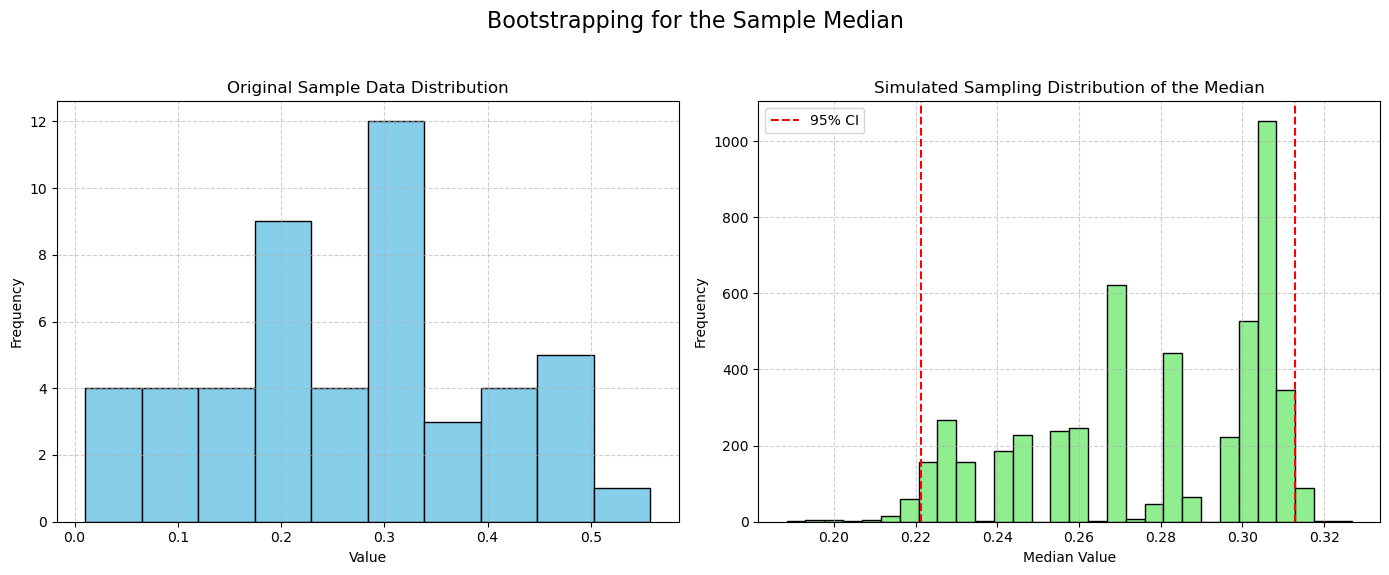
As can be seen, the resulting confidence interval spans over the values of high concentration of our sample.