Root finding algorithms

In numeric analysis root finding is equivalent to finding zeros of a continuous function. In case of complex and composite function finding values of a variable at which a function evaluates to zero is not a straightforward task, and thus root finding algorithms provide various iterative techniques for approximation of the root. In general root finding algorithms do not find all possible roots of a function but only the closest one to the initial guess (if any at all). Failing to find a root with approximation does not mean however that the function does not have any.

Newton’s method

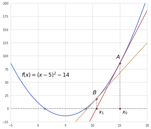
Newton’s method could be effectively used for root finding by making a linear approximation using first-order information (by taking the derivative) at a particular point. More details on how it actually works can be found here. It’s worth mentioning that Newton’s method may not converge if the starting point is far off from the actual root.

Bisection method

This is one probably the simplest method in root finding which starts off with two guesses where a function has values of opposite signs, say $f(a)$ is a positive and $f(b)$ is a negative value. The interval [$a$, $b$] is repeatedly bisected with a new point $c$ in the middle of it. After each bisection we either have $f(a) > 0$ and $f(c) \leq 0$ or $f(c) \geq 0$ and $(b) < 0$. The interval with opposite signs is selected and the procedure is repeated all over again until the interval becomes small enough, in which case the root is considered to be found. Although this algorithm is robust it might be too slow.

Secant line method

This method assumes that the function is approximately linear in the region of interest. It starts off with two initial guesses and puts a line between them (a secant line). In each next iteration the point where the secant line reaches zero is selected as a new one which substitutes the first point in the previous pair of guesses.

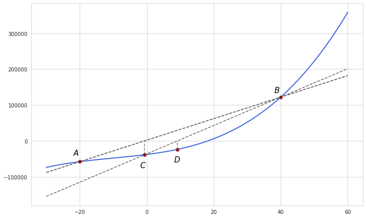
In the example above points $A$ and $B$ are selected as initial guesses whereas $C$ and $D$ were the ones found in the next two iterations. In this particular example convergence towards the visible root is not likely which is the problem with the secant method. Although it’s generally faster than the bisection method, it usually fails to converge if the initial guesses are not sufficiently close to the root.

Having two points the slope of the secant line can is determined in the following way:

     $a = \frac{f(x_1)-f(x_0)}{x_1 - x_0}$

And then the intercept is easily found as

     $b = f(x_1) - ax_1$

Putting it all together the equation for the secant line can be expressed like this:

     $f(x) = ax + b = \frac{f(x_1)-f(x_0)}{x_1 - x_0}(x-x_1) + f(x_1)$

From here the new point where the secant line reaches zero is determined with this formula:

     $x_2 = x_1 - f(x_1)\frac{x_1 - x_0}{f(x_1)-f(x_0)}$

The formula is actually similar to the one used in Newton’s method; only the slope based on difference is used instead of the one obtained from the derivative.

There is an improvement to this method known as false position method (or regula falsi) which makes sure that the algorithm converges by selecting points where a function assumes different signs, as opposed to selecting the last point regardless of its sign.

A generalization of the secant method in multidimensional space is known as Broyden’s method which is described in greater details here.

Inverse quadratic interpolation

This method works by taking three initial guesses and constructing a Lagrange polynomial which goes through each of these points (more about Lagrange interpolation can be found here). The polynomial here is “inverted” because instead of making an approximating function of $x$ which finds values of $y$ we want to make a function of $y$ which finds a value $x$. By setting $y=0$ we can find a single root of this polynomial.

Here is the general form of Lagrange polynomial if we have three points:

     $g(y) = \frac{(y-y_{i-1})(y-y_{i})}{(y_{i-2}-y_{i-1})(y_{i-2}-y_{i})}x_{i-2} + \frac{(y-y_{i-2})(y-y_{i})}{(y_{i-1}-y_{i-2})(y_{i-1}-y_{i})}x_{i-1} + \frac{(y-y_{i-2})(y-y_{i-1})}{(y_{i}-y_{i-2})(y_{i}-y_{i-1})}x_{i}$

And setting $y=0$ we obtain an equation for finding $x_{i+1}$:

     $x_{i+1} = \frac{y_{i-1}y_{i}}{(y_{i-2}-y_{i-1})(y_{i-2}-y_{i})}x_{i-2} + \frac{y_{i-2}y_{i}}{(y_{i-1}-y_{i-2})(y_{i-1}-y_{i})}x_{i-1} + \frac{y_{i-2}y_{i-1}}{(y_{i}-y_{i-2})(y_{i}-y_{i-1})}x_{i}$

This method is generally unreliable, and as it fails if two values of $y$ match. However it is used as a special case within Brent’s method which is discussed further.

Brent’s method

This a hybrid method which combines besection, secant line and inverse quadratic interpolation. Since the secant line method generally has a higher convergence rate than the bisection method we would like to use it whenever possible. At the same time we would like to switch to bisection if secant line does not lead to sufficient progress in root finding.

At first two initial values $a$ and $b$ are selected so that $f(a)$ and $f(b)$ have different signs and $f(b)$ is closer to zero than $f(a)$.

For the fallback bisection method we calculate $m$ as a midpoint between $a$ and $b$.

Furthermore, Brent’s method also introduces application of inverse quadratic interpolation whenever possible as it is slightly more efficient than secant line method. In order to proceed with the inverse quadratic interpolation the last three points should be different. Otherwise the secant method is checked.

The resulting value of interpolation $s$ should be between $b$ and $\frac{3a+b}{4}$. This ensures that our new step is certainly within the range of $a$ and $b$ and also not in the quarter closest to $a$ so presumably the new point is good enough. If this condition is not satisfied then the bisection method is applied.

A couple more conditions are imposed in order to handle ill-behaving functions. First of all, the new step should be greater than some small number - a tolerance level. If it is not then bisection is used over interpolation. If bisection was used at the previous step then the algorithm checks if the distance between the new point $s$ and point $b$ is smaller than half of the distance taken during the previous step. If it is not then bisection should make better progress. Similarly, if interpolation was used at the previous step then the distance between the new point $s$ and point $b$ should be smaller than half of the distance taken during the step before the previous one. If not then bisection is done as well.

According to the secant line mechanism we should use these two points at first, and in the future iterations - last two points obtained in the previous step (also with the different signs).

On the whole, Brent’s method is at least as good as the bisection method, there is a guarantee that it will converge, and at the same time with sufficiently smooth functions it benefits from higher convergence rate of secant line and inverse quadratic interpolation.