Newton’s method

Similarly to gradient descent, Newton’s method is used for finding a minimum of a function through iterations. Unlike gradient descent however, it uses a second order derivative of a function, which provides additional information about its curvature, so that the algorithm can navigate faster towards the minimum of the function.

Newton’s method for root finding

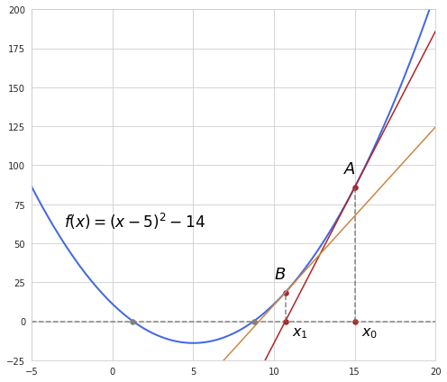
In order to better understand how the formula for Newton’s optimization works let’s take a look at a simpler problem: finding zero of a function. Suppose we have a simple function like this:

Finding zeros of this function is a trivial task which is easily solved analytically but it is also easy to demonstrate with this example how Newton’s method works as it may be similarly applied in more complex cases.
So first of all we have a starting guess for the value of $x$, in our example it’s 15 (the value of $x_0$), which corresponds to the value of the function at point A. From here we make a linear approximation of the function using derivative at that point and see where this approximation reaches zero. Following the example above, we see that the derivative becomes zero at point $x_1$ which is closer to the point of the original function’s zero. After that the procedure is repeated a number of times until we get sufficiently close to zero. In our example the second approximation is performed from the point B, and we see that the zero point of this approximation is very close to the original function’s point of zero.

Let’s take a closer look at what happens at each iteration. The derivative of a function at a certain point represents the slope of a function at that particular point or a tangent of the angle between $x$-axis and the slope line. If we look at the triangle formed by points A, $x_0$ and $x_1$ we see that it’s a rectangular triangle. The tangent is then equivalent to the relation between lengths of A$x_0$ and $x_1 x_0$. The length of A$x_0$ is just the value of the function at point A, and the length of $x_1 x_0$ is the actual update step during the iteration.

     $f’(x_0) = \frac{f(x_0)}{x_0-x_1}$

From here with some rearrangement we get the final formula for the updated step:

     $x_t = x_{t-1} - \frac{f(x_{t-1})}{f’(x_{t-1})}$

Newton’s method for optimization

So now when we know how to find zero of a function finding a minimum would seem like a small modification of the algorithm. Recall that the derivative of a function is zero at its critical points. Knowing that we can apply the same technique, only instead of finding zero of a function using derivative we shall find zero of the derivative using the second derivative as approximation.

We start off with approximation of a function at some initial point A with the second-order Taylor expansion which will produce quadratic function $\phi(x)$ like this:

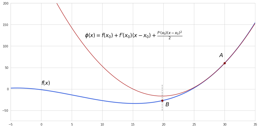
Next step is finding the point where approximation $\phi(x)$ reaches its minimum, that is the point where the derivative of this approximation is zero. Also we can check if we are moving in the right direction by looking at the second derivative - if it’s positive then we are at a minimum of the approximation.

     $\frac{d}{d (x-x_0)}(f(x_0) + f’(x_0)(x-x_0) + \frac{1}{2}f’’ (x_0)(x-x_0)^2) = 0$

     $f’(x_0) + f’’ (x_0)(x-x_0) = 0$

     $x - x_0 = - \frac{f’(x_0)}{f’’ (x_0)}$

From here we get a very similar equation to the one of zero finding:

     $x_t = x_{t-1} - \frac{f’(x_{t-1})}{f’’ (x_{t-1})}$

Same as in gradient descent, the procedure is repeated util the algorithm reaches a point sufficiently close to the true minimum of a function. In our example just in single step we approached pretty close to the minimum of the original function.

Multivariate optimization

In practice we usually have to deal with functions of multiple variables of course. The second-order Taylor expansion for multivariable function $f(x)$ takes the following form:

     $\phi(x) = f(x_0) + \nabla f(x_0)^{T}(x-x_0) + \frac{1}{2}(x-x_0)^{T}Hf(x_0)(x-x_0)$

where $\nabla f(x_0)$ is a vector of partial derivatives at the centering point (the gradient) and $H f(x_0)$ is a matrix of partial second derivatives (Hessian matrix) at that point.

Eventually the equation for finding the minimum will transform into this:

     $x_t = x_{t-1} - [H f(x_{t-1})]^{-1} \nabla f(x_{t-1})$

Applying the inverse of the Hessian is like dividing by the second derivative in our equation for for univariate optimization.

The actual Hessian however might not be invertible and in this case it would have to be modified, for example by adding a multiple of the identity matrix to it. Or we could just switch to gradient descent instead.

If the original function is twice differentiable at each point of interest then according to Schwarz’s theorem the order of differentiation by different variables does not matter, which means that the Hessian is a symmetric matrix. In addition, the found critical point is a minimum only if the Hessian is a positive definite matrix. A symmetric positive definite matrix has real and positive eigenvalues, meaning that the linear transformation encoded in this matrix represents moving in positive direction along each of the eigenvectors. Regarding our function approximation, only the point of minimum satisfies the condition that moving in any direction from it will be seen as ascending. If the Hessian is not positive definite (for example when we have both positive and negative eigenvalues) then the convergence will be towards a saddle point which is not what we want. More about symmetric and positive definite matrices can be found here.

Although Newton’s method is faster in terms of convergence it is computationally expensive, mainly due to the need to calculate the Hessian and its inverse. Quasi-Newton methods are designed to combat this issue by calculating only approximations of the Hessian.