Loss functions
In machine learning the loss function (or cost, or cost function) is something that lets the machine to actually “learn”. The loss function is the function of parameters, it evaluates the error of a model by comparing each predicted result with the actual observed data, thus measuring the residuals for different sets of parameters. Then it aggregates all individual residuals and comes up with a single value which generally describes how badly the function fits to the actual input data: the greater the value of the loss function - the worse is the model. Using different optimization techniques the loss function is minimized to a reasonable extent, thus making a machine learning model better.
Depending on specific situations, different types of the loss function may be employed. Among the factors that help to choose which loss function to use are the type of machine learning model, the presence of outliers, complexity of calculating the derivatives, and some prior knowledge about the model.
Usually the loss function is a realization of some distance metric, for example the sum of all distances across all of the training datapoints.
In a broad sense, with respect to the type of machine learning problem, the two main categories are regression losses and classification losses. This article should serve as an outline for the most used ones.
Regression losses
Mean squared error/quadratic loss/L2 loss
The mean squared error (MSE) is the average of the squared distances between predicted and observed values.
$MSE = \frac{\sum_{i=1}^n (\hat{y} - y_i)^2}{n}$
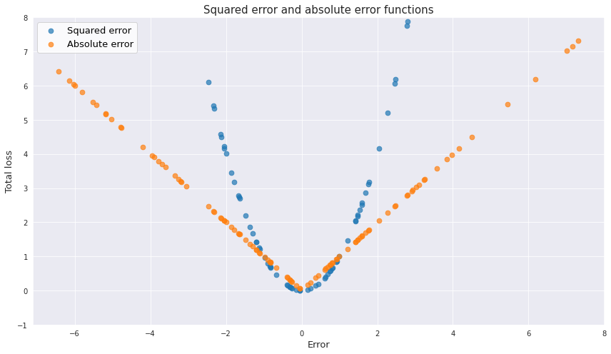
This function results in a single positive number regardless of the direction of the error. In addition, squaring bigger residuals produces even bigger values for the loss function, therefore, the function heavily penalizes significant deviations of the model compared to the lesser ones. So to speak, missing by a little lots of times is considered better than missing by a lot a few times. One has to be careful when applying this function to the data with outliers.
Other than that, the function has nice mathematical properties, in particular regarding calculation of gradient descent, since calculation of a derivative of quadratic function and finding the point of its minimum is quite straightforward. An overview of numerical methods for minimizing this particular loss function can be found here. Back to top ↑
Mean absolute error/L1 loss
The mean absolute error (MEA) is the average of the absolute distances between predicted and observed values.
$MAE = \frac{\sum_{i=1}^n |\hat{y} - y_i|}{n}$
Like MSE this function does not consider the direction of errors and always results in a positive number, and it is more robust to the effect of outliers. Below is the visualization of the effect that both MSE and MAE have on the residuals.
And yet, MAE is harder to use because the gradient descent cannot be applied to it (the problem with the point of discontinuity at the origin). Back to top ↑
M-estimators
This is a general family of loss functions which were designed to be both robust to outliers and be easier to optimize with gradients. M-estimators consider some general function of residuals $H(\varepsilon)$ and then minimize the sum of this function.
$S = \sum_{i=1}^n H(\varepsilon_i) = \sum_{i=1}^n H(\hat{y} - y_i)$
Actually the mean squared error function can also be viewed as an M-estimator where $H(\varepsilon)=\varepsilon^2$. However for better robustness properties other functions of residuals are used instead. A good candidate for $H(\varepsilon)$ should have certain properties which a needed for being able to calculate the minimum of the function:
- Non-negative
- $H(0) = 0$
- Symmetric, $H(-\varepsilon_i) = H(\varepsilon_i)$
- Monotonic, that is if $\lvert\varepsilon_i \rvert > \lvert\varepsilon_j \rvert$ then $H(\varepsilon_i) > H(\varepsilon_j)$
- Continuos - we need to be able to calculate the derivative with respect to the parameters of the regression so that the minimum could be found. This is the property which MAE does not have
So in case of the general form of the error function, the derivative with respect to $k$th parameter takes the following form after applying the chain rule:
$\frac{\partial S}{\partial \theta_k} = \sum_{i=1}^n \frac{\partial H}{\partial \varepsilon_i} \frac{\partial (\theta_k x_i - y_i)}{\partial \theta_k} = \sum_{i=1}^n \frac{\partial H}{\partial \varepsilon_i} x_{ki}$
This expression is set to be equal to zero and solved for all parameters simultaneously. In the general case the values of the parameters are calculated through the iterative reweighting procedure. It is done by defining a “weight” variable as
$w_i = \frac{1}{\varepsilon} \frac{\partial H}{\partial \varepsilon_i}$
So in this case
$\frac{\partial S}{\partial \theta_k} = \sum_{i=1}^n w_i \varepsilon_i x_{ki} = \sum_{i=1}^n w_i (\theta_k x_i - y_i) x_{ki} = 0$
All the weights are set to be equal to some guess variable, for example to 1, and then we have a system of linear equations which can be easily solved for $\theta$. Using the newly found values of $\theta$ the error terms are calculated as well, and then using the function of error $H(\varepsilon)$ a new set of weights $w$ is calculated. The whole procedure is repeated until the convergence is reached.
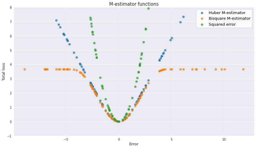
There are a few notable functions which may be used as the residual function. Historically the first was the Huber M-estimator which looks like this:
\[\begin{cases} \frac{\varepsilon^2}{2} & \text{for} \left|\varepsilon\right| \leq k, \\ k\left|\varepsilon\right| - \frac{k^2}{2} & \text{for} \left|\varepsilon\right| > k \end{cases}\]For errors which are not bigger than some threshold this function behaves more like the mean squared error, which ensures that the function is continuous at the origin. In case of bigger errors the function behaves more like the mean absolute error, and the penalization of the outliers becomes proportional to their distance to the mean. As for the $k$ value, Huber proposed 1.345 of standard deviation of a sample, which results in approximately 95% of efficiency which MSE provides.
Another common error function is bisquare M-estimator:
\[\begin{cases} \frac{k^2}{6} (1-(1-(\frac{\varepsilon}{k})^2)^3) & \text{for} \left|\varepsilon\right| \leq k, \\ \frac{k^2}{6} & \text{for} \left|\varepsilon\right| > k \end{cases}\]This type of function is even more robust than the Huber M-estimator. For the residuals with the values greater than some threshold (the proposed value for $k$ is 4.685 standard dviations) the penalization remains constant.
Classification losses
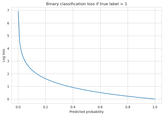
Cross-entropy
This is a go-to loss function which is used in classification. In order to understand it let’s first see what entropy is.
Entropy is the measure of randomness of a system. With respect to classification in machine learning, high entropy means high uncertainty as to which particular class an observation belongs to. For example, when rolling a fair dice the entropy is high because no matter what the target outcome is, its probability will be just 1/6, so we are generally uncertain about it. On the contrary, the entropy is low if we have high confidence about a particular outcome, for example we may be 90% certain that a certain dog belongs to a certain breed based on its appearance.
The entropy measure has a number of requirements to satisfy:
- The uniform distribution should have higher uncertainty than any skewed one; at the same time the uniform distribution with more outcomes has even greater entropy.
- The entropy is additive to independent events. The outcome of one event does not help in predicting the outcome of an independent event.
- Inclusion of the event with zero probability has no effect on the general entropy. On the contrary, the events with completely certain outcomes have zero uncertainty.
- The measure of uncertainty is continuous.
In order to understand the entropy better let’s also introduce the concept of surprise. Surprise is a measure which is opposite to probability: it is small if the probability is high, and vice versa. The surprise is not equal to the reciprocal of probability but instead is made to be a convenient construct for the requirements of the entropy: $\log \frac{1}{p(x)}$, where $p(x)$ is the probability. The entropy is the expected value of surprise for all possible outcomes:
\[H(X) = \sum_{x\in {\mathcal {X}}} p(x)\log \frac{1}{p(x)} = - \sum_{x\in {\mathcal {X}}} p(x)\log (p(x))\]Application of the idea of entropy and surprise in classification loss is knowns as cross-entropy:
\[H(p, q) = - \sum_{x\in {\mathcal {X}}} p(x) \log (q(x))\]where $p(x)$ is the observed probability of a certain category $x$, and $q(x)$ - its predicted value.
Similarly to the entropy formula, the cross-entropy calculates the average surprise for the predicted categories in terms of their true probabilities. Intuitively, the loss is naturally increased if the model assigns high surprise for a category whose real observed share is not small (not surprising). The greater the distance from the true observation probability - the greater the loss.