Line search

Generally speaking, line search is one of the two (the other is trust region) major strategies in non-linear optimization. Line search methods first determine the direction in which to move the value of the parameter and then perform calculations in order to select the appropriate step size which will produce sufficient decrease in the objective function. In iterative optimization algorithms the step size might be either too short, leading to a slow convergence towards the minimum of the loss function, or too long which results in overshooting the minimum on each iteration. Line search hence aims at reducing the number of iterations before convergence by selecting the appropriate step size at each pass. In gradient descent for example line search could be used for determining the proper learning rate.

In practice however, line search is rarely used because determining the step size at each iteration adds computational overhead which outweighs the relative benefit of fewer iterations. In addition, line search in stochastic methods will only determine the optimal step for an approximation which is not really useful. Yet it is useful to understand the ideas behind the line search methods as it may help in understanding other techniques in optimization.

Search direction

The direction of the parameter change is determined by the direction of the steepest descent, that is by taking the derivatives of a function with respect to each parameter at a given point. Since the direction does not provide information about the length, the vector of the derivatives should be scaled accordingly. So the formula of the search direction in case of gradient descent at step $k$ will be as follows:

     $d_k = \frac{-\nabla f_k}{\left|\left|\nabla f_k\right|\right|}$

If the derivative $\nabla f(x_k)$ is positive then we have an upward slope, so in order to move towards the minimum we need to move back along $x$ axis - $d$ becomes negative. Similarly, if $\nabla f(x_k)$ is negative - we must use positive $d$.

For the conjugate gradient descent the search direction will be determined like this:

     $d_k = -\nabla f_k + \beta_k d_{k-1}$

where $\beta$ is a coefficient that enforces $d_k$ and $d_{k-1}$ be conjugate.

Other options are Newton or quasi-Newton search directions.

     $d_k = - \nabla^2 f_k^{-1} \nabla f_k$ or $d_k = - B_k^{-1} \nabla f_k$

where $B_k$ is an approximation of a Hessian matrix.

Step size

Although line search methods should provide the possibility to converge in fewer steps, we do not want to spend too much time determining the optimal step size at each iteration.

One highly impractical method is performing exact line search which tries to find the exact step size for bringing the function to the minimum. For example, in case of gradient descent the new point is determined like this:

     $x_t = x_{t-1}- \eta\nabla f(x_{t-1})$

Under the exact line search the optimal learning rate would be selected as such that ensures minimum value for $f(x_t)$, so we need to find the derivative of $f(x_{t-1}- \eta\nabla f(x_{t-1}))$ with respect to $\eta$, set it equal to 0, and evaluate for $\eta$.

Instead of finding the step size which will ensure moving to the exact minimum of the objective function is usually enough to find an approximate step which will move sufficiently close to the minimum, hence inexact line search methods are more preferred as they require less computations.

There are two conditions, called Wolfe conditions, which are considered in order to determine the sufficient step size. The first condition, also known as Armijo rule, ensures that the step length leads to sufficient shift towards the minimum of the objective function:

     $f(x_k + \eta_k d_k) \leq f(x_k) + c_1 \eta_k\nabla f(x_k)d_k$

where $\eta$ is the step size at point $k$ and $c_1$ is a small number between 0 and 1.

This is the graphical representation of an function which is dependent on the step size:

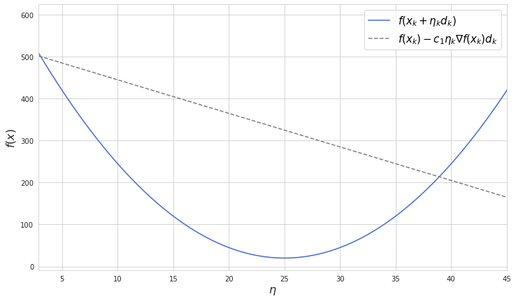
As long as we select $\eta$ less than the point where two lines are crossing the Armijo rule will be satisfied, while further bigger steps will be considered too big.

If we select $c_1$ to be equal to 0 then $f(x_k) - c_1 \eta_k\nabla f(x_k)d_k$ will become a horizontal line. In this case it is possible to make such a step which will overshoot the minimum and land at an identically distant point, so the convergence is not guaranteed. If we take $c_1$ equal to 1 then $f(x_k) - c_1 \eta_k\nabla f(x_k)d_k$ will just become a tangent line which will not allow any step according to the Armijo rule. Generally taking $c_1$ closer to zero gives more freedom for selecting the step size.

While the first Wolfe condition rejects too long steps, the second one aims at preventing too short steps. We know that at the point of the minimum the derivative of $f(x_k + \eta_k d_k)$ is zero. Yet as opposed to the exact line search we would be happy to make a sufficiently long step which does not necessarily land at the minimum. The derivative at the new step should be less than the derivative at the previous one and the relationship between them needs to be less or equal than some variable variable $c_2$ which is between 0 and 1:

     $\frac{\nabla f(x_k + \eta d_k)d_k}{\nabla f(x_k)d_k} \leq c_2$

On rearrangement we get the equation for the second Wolfe condition:

     $\nabla f(x_k + \eta d_k)d_k \geq c_2 \nabla f(x_k)d_k$

The sign is changed because $\nabla f(x_k)d_k$ is always negative.

If we select $c_2$ close to 0 then we would force line search to look for a solution which is close to the minimum, while $c_2$ is closer to 1 then the search is less demanding. In order to apply both Wolfe conditions and ensure existence of $\eta$, $c_2$ needs to be selected greater than $c_1$.

Typically line search algorithms are done in two stages: bracketing, which finds the maximum possible step length, and interpolation, which computes a good step within it.

Backtracking line search

This type of line search is considered as a base method for other inexact line searches, and it makes use only of the first Wolfe condition. The algorithm starts with an initial relatively large guess for $\eta$ and then tests whether it satisfies the Armijo rule. If the step size is deemed as too big the next estimate of $\eta$ is selected like:

     $\eta_{n+1} = \tau \eta_n$

where $\tau$ is a reducing factor which is between 0 and 1.