Kernels overview
In this article
What are kernels
In statistics, a kernel typically refers to a window function used in various estimation techniques, such as kernel density estimation(KDE) and Gaussian process.
Being a window function means that it is applied to a certain region of values. Any region has a central point, and all other points around it are weighted in such a way that reflects their closeness to the central point.
Typically kernel functions are not used by themselves but rather are incorporated into other functions where they perform reweighting of the initial observations. The weight of each individual point is spread around the region around it whereas the center of the kernel is placed on that point.
A kernel function is a non-negative and symmetric function centered at 0. It also integrates to 1 over its support region which ensures that the total weight remains the same before and after reweighting.
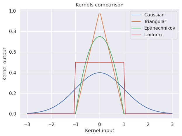
Commonly used kernel functions include:
- Gaussian (normal) kernel: $K(x)=\frac{1}{\sqrt{2 \pi}} e^{-\frac{1}{2}x^{2}}$.
- Epanechnikov kernel: $K(x)=\frac{3}{4}(1−x^{2})$ if $∣x∣\leq 1$, otherwise, otherwise 0.
- Triangular kernel: $K(x)=(1−∣u∣)$ if $∣x∣\leq 1$, otherwise, otherwise 0.
- Uniform (rectangular) kernel: $K(x) = \frac{1}{2}$ if $∣x∣\leq 1$, otherwise, otherwise 0.
Kernel density estimation
Kernel density estimation (KDE) is a technique used for estimating the probability density function of a random variable. The fundamental problem KDE addresses is data smoothing: making inferences about the population based on observed data.
KDE does not assume any parametric distribution. Instead, each datapoint from the sample is considered as an individual distribution and thus its value is substituted by a continuous distribution function (probability density) according to the selected kernel. The kernel input $x$ from the formulas above is the distance between an observed point and $x_i$ and any arbitrary point in its surrounding region. All of the resulting distributions are added together across the whole observed range of values, and thus the overall shape of the combined distribution is built.
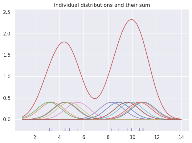
The choise of the kernel function in KDE does not really matter. The Gaussian kernel is used the most because it is infinitely differentiable. What’s more important is the selected bandwidth.
The bandwidth parameter determines the length scale of the kernel and therefore influences the smoothness of the estimated density. A larger bandwidth results in a smoother estimate because more neighboring points have impact on one another. On the other hand, a smaller bandwidth can lead to more variability in the estimate.
Here is how the formula for the kernel density estimation:
\[\hat{f}_h(x) = \frac{1}{n} \sum_{i=1}^n K (x - x_i) = \frac{1}{nh} \sum_{i=1}^n K \left(\frac{x - x_i}{h}\right)\]where $K$ is the kernel function, $h$ is the bandwidth.
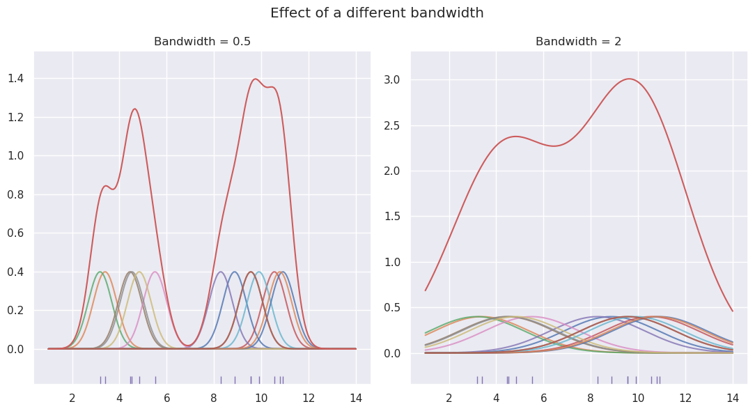
Since each individual distribution is integrated to 1, the combined sum of all distributions around the known points is divided by $n$ in order to make it equal to 1 as well. Notice however that the function also is scaled by the factor of the bandwidth $h$. This is because when including this factor into the kernel function, the area under the individual point distribution is multiplied accordingly. Therefore, in order to restore the overall sum of distributions to 1 it also needs to be divided by $h$.
Kernels in Gaussian process
In scope of the Gaussian process the kernels takes input of two numbers and produces the measure of their similarity. Thus they define the behavior of the resulting function distribution.
Kernels may be combined by adding or multiplying them together.
The result of adding kernels has the same effect on the covariance matrix as the addition of matrices. So for example if any of the two kernels which are added together produces the high number - the correlation between the two points is high. Usually noise is added to the kernel of a choice in order to prevent overfitting. As a consequence, the resulting mean function is no longer forced to pass through each observed point, and becomes more flexible.
In case of kernel multiplication the correlation between the two points is high if either of the individual kernels produces high correlation.
Let’s take a look at the commonly used kernels and see which effects their hyperparameters have.
Squared exponential kernel
Also known as Radial basis function (RBF) kernel, this kernel is infinitely differentiable, and has only two hyperparameters which eventually produces a nice-looking smooth function.
$k(x_i, x_j) = \sigma^2\exp\left(-\frac{(x_i - x_j)^2}{2\ell^2}\right)$
The hyperparameter $\sigma^2$ corresponds to the magnitude of deviations of the function’s values from its mean by scaling the covariance matrix appropriately. In other words it represents the level of uncertainty at unobserved areas.
The hyperparameter $\ell$ is the length scale factor which determines how long the correlation between the two points lasts, and so, how far the effect of a certain observation impacts the shape of a function in the neighboring areas. Increasing $\ell$ makes an effect of higher similarity for the two points which would otherwise be considered distant.
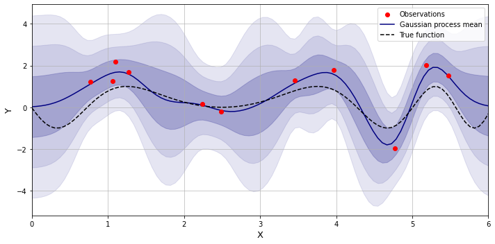
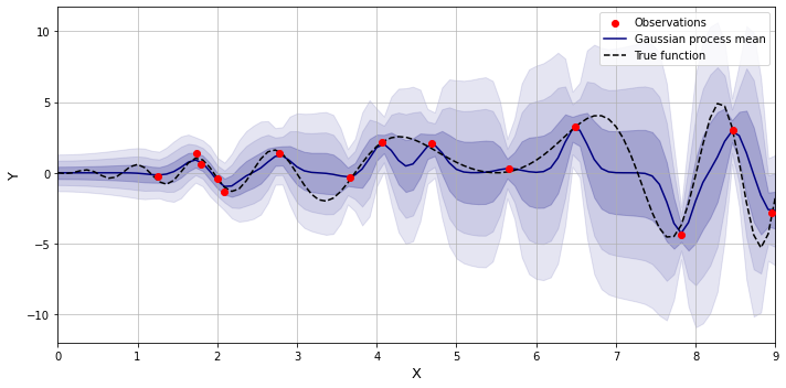
Below is an example of the function estimation with the squared exponential kernel with some added noise.
Matern kernel
This kernel is a generalization of the RBF kernel, which has an additional hyperparameter $\nu$ which defines how many times the resulting function may be differentiated. If $\nu$ is set to infinity then the kernel converges to the RBF kernel, however a popular choice of its value is 1.5 which makes the resulting function differentiable at least once, and in shape more realistic to the physical processes.
Periodic kernel
This kernel is also known as exponential sine-squared, and it allows modeling periodic processes.
$k(x_i, x_j) = \sigma^2\exp\left(-\frac{2 \sin^2 (\pi \lvert x_i - x_j\rvert / p)}{\ell^2}\right)$
In addition to the parameters already present in the RBF kernel, it also has the hyperparameter $p$ which adjusts the periodicity of the function.
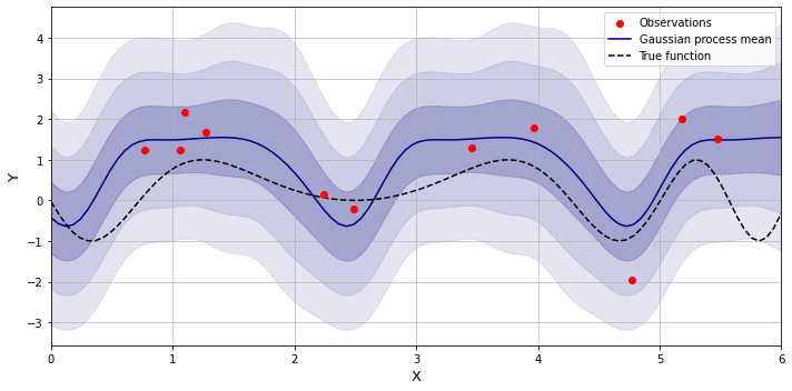
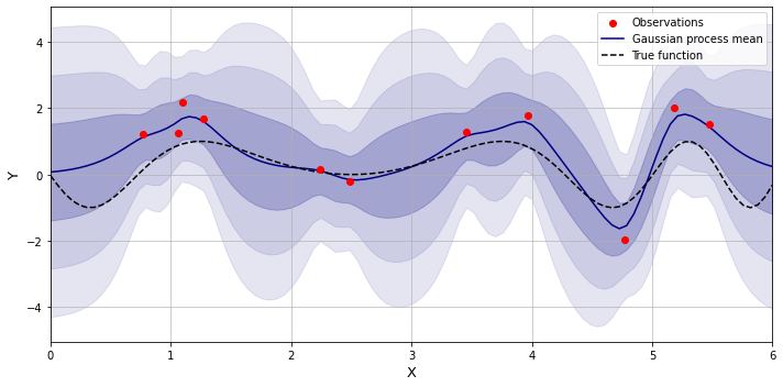
By taking the product of the squared exponential kernel and the periodic one, we may get a function of a periodic nature which yet varies over time.
Dot product kernel
Also known as the linear kernel, it belongs to a family of so-called non-stationary kernels where the measure of similarity depends not only on the relative distance between the two points but also on the absolute values of the coordinates.
$k(x_i, x_j) = \sigma^2 + x_i \cdot x_j$
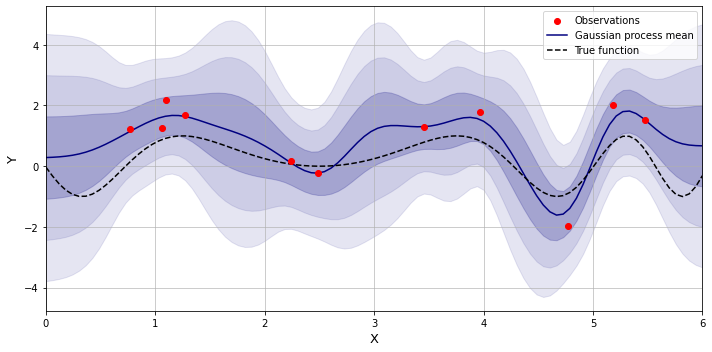
On its own this kernel produces just a straight line so it is used in combination with other kernels, when some sort of trend needs to be represented. Below is an example of adding the linear kernel to the periodic one.
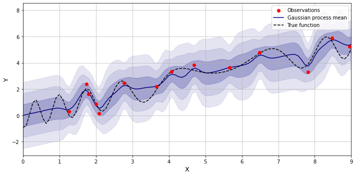
The product of the linear and periodic kernels produces a periodic function with ever increasing amplitude.
