Gradient descent

Gradient descent is bread and butter of machine learning. It is a fundamental method of finding the minimum of the loss function in neural networks, hence it is widely used in loss function analysis and optimization.

The mechanism of gradient descent

As we know, the derivative describes the slope of a function or the way the function changes when the predictor value changes. If the derivative of a function is negative at a certain point then the function at this point is decreasing. Also, the derivative of a function equals to zero when the function is at its critical points - local and global minima and maxima, as well as saddle points. Starting from a random point gradient descent searches for a minimum of a function by iteration through the following steps:

1. Measuring the derivative at its current point and comparing it to zero.
2. Multiplying the derivative by a small number called learning rate, so that a step size is determined.
3. Subtracting step size from the current point so that a new point is selected.

Here is a simple example of gradient descent towards a local minimum of a function.

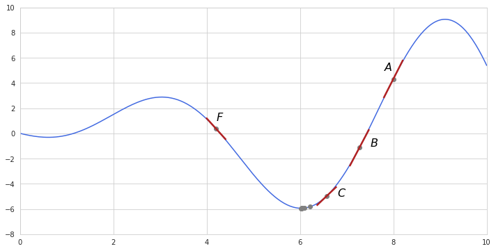
Starting from randomly selected point $A$ the derivative shows upward slope - the derivative of the function is positive and high. Multiplying this high number by the learning rate results into reduced but still substantial step size. Subtracting this step size from the previous point gets us to point $B$. The slope at $B$ is still high so another step is also quite significant - we move to point $C$. Now it becomes obvious that the slope is getting lower, so multiplying it by the learning rate results in a smaller step size during each following iteration. One of the nice things about gradient descent is that it takes larger steps when the slope is far from zero and very small steps when it approaches the minimum of a loss function. Decreasing step size ensures that gradient descent doesn’t overstep the function’s minimum, however as it reaches the minimum the slope becomes almost unnoticeable - so is the step size, which in turn leads to a very high number of iterations and computation cost which is undesirable. Setting a stopping criteria is useful in cutting the number of iterations. Such criteria may be simply the total number of allowed iterations or a point where the slope is close to zero meaning that further steps lead to insignificant improvements.

If we had selected a starting point with the negative slope, as at point $F$, then its derivative would be also negative. Subtraction of a negative number is equal to adding so essentially we would have moved in the positive direction in finding the function’s minimum. Thus in addition to adapting step size gradient descent by itself determines in which direction to move - doesn’t it sound cool?

Usage in loss function

Recall that the loss function is a function of parameters, and it measures the sum of residuals, telling how good a model is fit to data. The model is optimized when its set of parameters ensures that the sum of residuals is minimal, which is the same as when the loss function is at its minimum. Gradient descent can be used for exactly this purpose - finding such parameters at which the loss function reaches its minimum. Gradient descent is also very useful when it is impossible or hard to find the optimal parameters analytically (e. g. by using least squares estimation).

Suppose we have an empirical distribution like this:

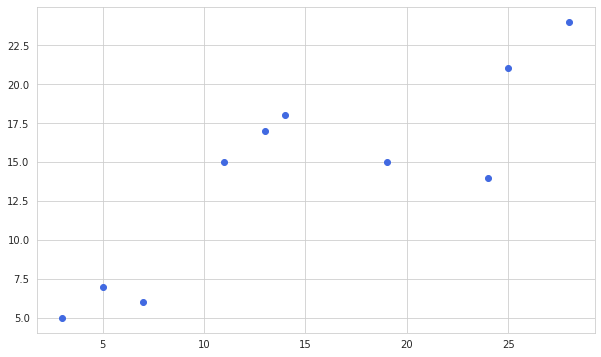
We want to find the parameters for a simple linear regression to this distribution:

     $f(x) = a + bx$

Suppose we already know the value of the intercept $a$, then we would only have to find such value of $b$, which minimizes the loss function (in this case mean square error but not necessarily so). Let’s start plugging different numbers for the slope and measuring the squared error of the estimation.

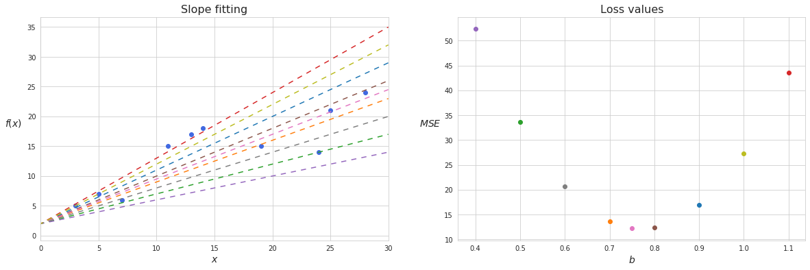
We can see that the shape of the loss function is actually a quadratic function, and that if we take $b$ between 7 and 8 then the loss function will be close to its minimum. There is, however, an infinitely large number of possible values for $b$ and calculating loss function for any single random guess would be simply overkill. Instead, we can apply gradient descent, and in a few iterations adjust the value of $b$ in such a way that the function of residuals gets pretty close to its minimum.

Multivariate gradient descent

In a more general case where a function is dependent on multiple input variables, for example if we need to estimate both $a$ and $b$ in the simple linear regression, the same logic with calculating derivatives for the loss function applies. However, in this case the loss function becomes multidimensional and instead of a single slope we need to find a direction in n-dimensional space in which to descend. The so-called multidimensional slope is determined by calculating partial derivatives with respect to each of the parameters, thus obtaining gradient (vector of slopes). Gradient is commonly depicted with $\nabla$, and here is how the gradient of loss function $J$ can be expressed:

\[\nabla J(\theta) = \left[\begin{array}{c} \frac{\partial J}{\partial \theta_1} \\ \frac{\partial J}{\partial \theta_2} \\ ... \\ \frac{\partial J}{\partial \theta_n} \end{array} \right]\]

where $\theta$ is a set of predictors representing $n$ dimensions. In case of finding a minimum of a loss function these predictors are parameters of the original function.

Going back to the overall procedure the formula for gradient descent may be constructed as follows:

     $\theta_t = \theta_{t-1}- \eta\nabla J(\theta_{t-1})$

where $\eta$ is the learning rate and $\theta_t$ is a new set of predictors.

Here is an example of gradient descent in two-dimensional space:

The area depicts the loss function values for all combinations of the parameters $\theta$ within certain scope. In order to simplify plotting, the loss function is usually projected on a two-dimensional plot of $\theta_0$ and $\theta_1$ with a contour plot, where each line represents areas where the loss function assumes the same value. Such areas of the same values are usually plotted with different colours, so that the areas of minima are easily distinguished. In the example above the areas where the loss function reaches its minimum are painted in blue.

Unfortunately, the best number which could be used as a value of the learning rate cannot be found analytically and thus has to be adjusted by trial and error. Smaller learning rates can lead to more precise estimations but would require more calculations while the bigger ones may lead to less accurate results, including overstepping the minimum of a function. Some techniques employed for finding the most appropriate learning rate include grid search, scheduling learning rate to decrease when a certain amount of steps is undertaken, and using adaptive learning rate.

Types of gradient descent

Typically gradient descent is applied to the loss function which is calculated using all available observations. This type of gradient descent is called batch gradient descent. It is quite stable and is guaranteed to converge to a local or global minimum depending on the initial guess for parameters, however for a large number of observations and parameters this type of gradient descent may be slow and computationally expensive.

Stochastic gradient descent (SGD) on the other hand instead of the whole dataset takes only one single randomly chosen point for calculating the loss, which significantly simplifies further calculations of the gradient. After the parameters are optimized for a loss function based on a single observation, the procedure is repeated a number of times for other randomly chosen points. The stochastic gradient descent is unstable, as each new point of observation may significantly change the parameters obtained at a previous step with a chance of overstepping a local minimum. This however may result in a better or even global minimum in case of non-convex functions. Below, on a contour plot we can see how stochastic gradient descent converges towards the minimum of a loss function.

One good practice for applying the stochastic gradient descent is to slowly decrease the learning rate so that the function will stop overstepping a point of minimum.

On the other hand, a modification of this algorithm called mini-batch stochastic descent takes several points (a subset) instead of a single one for calculating the loss function. Although the mini-batch stochastic descent is not as fast as the regular stochastic descent, it results in more stable convergence.

Enhancements to gradient descent

More recent studies proposed new methods of how the “classical” gradient descent may be improved. Slow convergence and the need to manually select and tune the learning rate are among the most discussed shortcomings. Here are some notable examples of these improvements.

Gradient descent with momentum

The problem this extension tries to tackle is slow convergence in the standard gradient descent. When the slope becomes too gentle gradient descent takes too small steps, has hardship escaping valleys and even may stop at a saddle point. In addition, the slope may be oscillating around the general direction of the slope following ravines in the loss function. Such ravines may change direction from one step to another, meaning that gradient descent will have to take zigzagging steps towards the minimum of the loss function. As we already saw, such oscillations may be caused by stochastic gradient descent when a new point of the original function tries to “correct” the parameters from the previous step.

The momentum allows us to reduce oscillations while also increasing the speed of convergence. One common metaphor for gradient descent is a man trying to descend the mountain in the direction of the steepest slope. However in order to understand the momentum it is better to modify this image to describe a ball rolling downhill. The force with which the ball rolls in the general direction does not allow it to change direction significantly when it encounters ravines, and the ball does not immediately slow down upon reaching a valley as it continues moving from accumulated momentum.

The momentum can be achieved by applying the concept of exponential moving average to the gradient.

     $V_t = \beta V_{t-1} + (1-\beta) S_t$

where $S_t$ is the value from a new observation, and $\beta$ is a coefficient of weight, which takes value from 0 to 1 and is responsible for determining which fraction of value to take from previous observations. For gradient descent with momentum $\beta = 0.9$ is a good choice. One way to view this equation is by making analogy with physics, where $V_{t-1}$ is velocity at the previous point, $\beta$ is air resistance due to which a part of velocity is somewhat decreased, and $S_t$ is acceleration added at new point.

The momentum works well for gradient descent because within the formation of the compound effect of gradients $V$ all oscillations from previous iterations largely cancel each other out. The new gradient, which is computed at each next step, accounts for the value $S_t$ in the equation of exponential moving average. For here with respect to gradient descent the moving average of all gradients can be expressed like this:

     $V_t = \beta V_{t-1} + (1-\beta) \eta \nabla J(\theta)$

Since the learning rate can be selected to account for $(1-\beta)$ term thus making it redundant, this term is usually omitted in the literature.

     $V_t = \beta V_{t-1} + \eta \nabla J(\theta)$

Then the gradient descent is calculated like this:

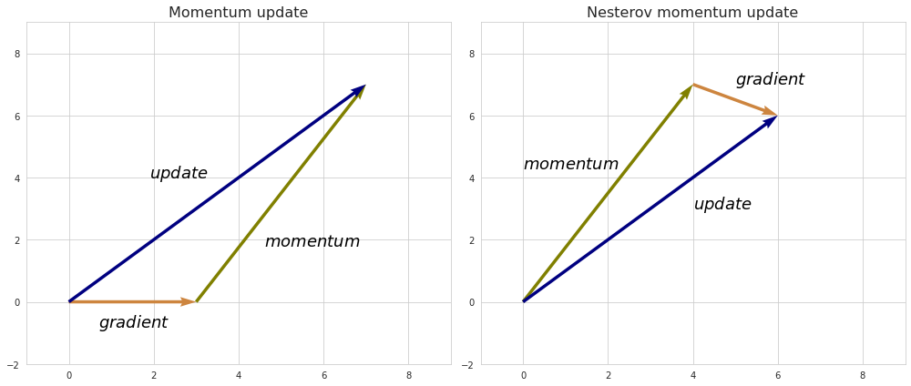
     $\theta_t = \theta_{t-1} - V_t$

Here is a display of SGD with momentum in comparison with vanila SGD:

An improvement to gradient descent with momentum, namely Nesterov accelerated descent (NAG), was introduced to prevent the descent from making too big steps when the direction of the slope changes. While gradient descent with momentum measures the slope of a loss function at its current point and then takes modified with momentum step in the direction of this slope, NAG instead measures the slope at the point where the momentum step alone would be applied so that it can check if the slope changes direction at its next point. The combined effect of the momentum and the look-ahead slope define the actual step of such descent. So to speak, the slope at the look-ahead point “corrects” the momentum force.

The formula for Nesterov accelerated descent would look like this:

     $V_t = \beta V_{t-1} + \eta \nabla J(\theta - \beta V_{t-1})$
     $\theta_t = \theta_{t-1} - V_t$

AdaGrad

Another issue which can be addressed in gradient descent is equal learning rate for all features and on each iteration. AdaGrad (adaptive gradient) extension to gradient descent provides a mechanism for automatic tuning of learning rate gradually reducing it, so that each next iteration of descent is less likely to overstep the minimum of a function.

In the related literature the gradient at a certain iteration is often depicted as $g_t$ instead of $\nabla J(\theta_{t})$. Updating of parameters under AdaGrad is done according to this rule:

     $\theta_t = \theta_{t-1} - \frac{\eta}{\sqrt{\sum_{\tau=1}^t g_{\tau}^2 + \epsilon}} g_t$

Here the denominator represents L2 norm of all previous gradients of the parameter up to the $t$-th iteration. $\epsilon$ is just a very small number which simply prevents denominator from being zero, and $\eta$ is a global learning rate set in advance.

Obviously adding another gradient causes the learning rate to decrease. In addition, larger gradients cause smaller learning rates and vice versa. Sparse features change slowly, hence their gradients are typically small. Applying a larger learning rate to them would lead to a similar scale of descent along each dimension.

AdaGrad extension is still sensitive to the choice of the global learning rate, so it has to be tuned through error and trial. Another significant problem is rapidly diminishing learning rate: after a certain number of iteration the number in the denominator becomes big enough so that individual learning rates become so small that the progress towards the minimum becomes nonexistent.

AdaDelta

AdaDelta was developed with a purpose to eliminate the shortcomings of AdaGrad. While AdaGrad uses accumulated sum of squares of all previous gradients in denominator which leads to rapidly diminishing learning rate, AdaDelta instead puts in denominator exponential moving average of squared gradients:

     $E\lbrack g^2\rbrack_t = \beta E\lbrack g^2\rbrack_{t-1} + (1-\beta) g_t^2$

Similarly to the equation of moving average used in momentum calculation $\beta$ is a coefficient of weight, which takes value from 0 to 1 and is responsible for determining which fraction of value to take from previous observations. In practice the choice of $\rho$ does not make a significant impact on the performance of the algorithm.

The square root of such exponential moving average used in denominator is known as root mean square (RMS) of all previous updates of parameters.

     $RMS[g]_t = \sqrt{E[g^2]_t + \epsilon}$

This improvement alone is known as RMSprop algorithm.

     $\theta_t = \theta_{t-1} - \frac{\eta}{RMS[g]_t}g_t$

Further on, in order to also remove the need to manually select global learning rate as in AdaGrad, AdaDelta uses RMS of previous parameters updates instead of the global learning rate, so that eventually the update rule for AdaDelta gradient descent looks like this:

     $\Delta \theta_t = - \frac{RMS[\Delta \theta]_{t-1}}{RMS[g]_t}g_t$

Using RMS of $\theta$ in numerator also solves the issue of different units in parameters update. The gradient shows the relation between change in the values of the loss function (which is unitless) and units of the parameters. Both the standard and momentum gradient descent basically evaluate to $1/\theta$ units and then use it in order to determine the magnitude of change in $\theta$ units. AdaGrad uses just unitless measure in order to determine the step in $\theta$ units. AdaDelta however has the units of gradient canceled with the units from denominator so that only numerator units of $\theta$ remain.

It is worth noting that RMS of $\theta$ should also include the value of $\epsilon$ in order to provide a starting value in calculation of the exponential moving average.

Adam

Adam (adaptive moment estimation) may be viewed as an extension to RMSprop algorithm where momentum is added to the gradient calculation. In its core Adam utilizes first and second order moments, hence the name. Both moments decay over time as in AdaDelta and RMSprop:

     $E\lbrack g\rbrack_{t} = \beta_1 E\lbrack g\rbrack_{t-1} + (1-\beta_1) g_t$
     $E\lbrack g^2\rbrack_t = \beta_2 E\lbrack g^2\rbrack_{t-1} + (1-\beta_2) g_t^2$

Then the update rule takes the following form:

     $\theta_t = \theta_{t-1} - \frac{\eta}{\sqrt{\widehat{E[g^2]_t} + \epsilon}} \widehat{E[g]_t}$

Adam makes bias correction for the moment updates as the initial values of the moments are close to zero. The bias correction increases their values at the beginning of iteration so that the algorithm picks up faster while later values remain almost unchanged.

     $\widehat{E\lbrack g\rbrack_t} = \frac{E\lbrack g\rbrack_t}{1-\beta_1^{t}}$
     $\widehat{E\lbrack g^2\rbrack_t} = \frac{E\lbrack g^2\rbrack_t}{1-\beta_2^{t}}$

The recommended default value for $\beta_1$ is 0.9, and for $\beta_2$ is 0.999.

A modification to Adam where it uses Nesterov accelerated descent instead of momentum is known as Nadam.