Expectation Maximization

The Expectation-Maximization (EM) algorithm is a powerful iterative method used in statistics to find the maximum likelihood or maximum a posteriori (MAP) estimates of parameters in statistical models. It is particularly useful when the model depends on unobserved, or latent, variables.

The Problem EM Solves

Directly finding the maximum likelihood estimates typically relies on taking the derivative of the likelihood function with respect to each parameter and setting it to zero. However, when a model contains latent variables, this approach becomes intractable. The presence of unobserved data introduces a complex summation or integral that makes the direct calculation of the derivative impossible to solve.

The EM algorithm provides an elegant solution by breaking this hard problem into two more manageable steps: an expectation step and a maximization step.

The Two Core Steps: Expectation and Maximization

The EM algorithm operates by iteratively improving an initial guess for the model parameters. Each iteration consists of two main steps:

Expectation (E) Step: In this step, the algorithm uses the current parameter estimates to compute the “expected” value of the log-likelihood function. This is done by calculating the posterior probability of the latent variables given the current parameters and the observed data. Essentially, the algorithm “fills in” the missing data with the most probable values given the current model.

Maximization (M) Step: The algorithm then treats the “expected” values from the E-step as if they were the true, observed data. It then finds new parameter estimates that maximize this new, simplified likelihood function. These new parameters are a better fit for the data and are used for the next iteration.

This two-step process repeats until the parameter estimates converge to a stable solution, which represents a local maximum of the likelihood function.

A Classic Example: Gaussian Mixture Models (GMM)

A classic application of the EM algorithm is in Gaussian Mixture Models (GMMs), a common clustering technique.

Imagine you have a dataset of points, but you don’t know which cluster each point belongs to. The cluster assignment is the latent variable. Our goal is to find the mean, variance, and weight of each cluster that best explains the observed data.

Here’s how EM solves this problem:

1. Initialize Parameters: Make an initial guess for the parameters of each Gaussian cluster (mean, variance, and the mixing weight).

2. E-Step (Soft Assignment): For each data point, calculate the probability that it belongs to each cluster, using the current parameter estimates. Instead of a hard assignment (e.g., “point 1 belongs to cluster A”), this is a “soft” assignment (e.g., “point 1 has a 70% probability of belonging to cluster A and a 30% probability of belonging to cluster B”). This fills in our missing cluster assignment data with probabilistic expectations.

3. M-Step (Parameter Update): Using the soft assignments from the E-step, update the parameters of each cluster. For example:

• The new mean of a cluster is the weighted average of all data points, where the weights are the soft assignment probabilities calculated in the E-step.
• The new variance is also calculated from the weighted data.
• The new mixing weight for a cluster is simply the sum of all soft assignment probabilities for that cluster.

These two steps are repeated. With each iteration, the cluster assignments become more certain and the parameters converge to a solution that best fits the underlying data structure.

The Mathematical Foundation

Now let’s see how it works and more importantly why it works.

In the most general sense, as per the maximum likelihood estimation we want to maximize the log-likelihood function $\log \mathcal{L}(\theta \mid X)$, which is equivalent of maximizing the probability of data given the parameters $\log P(X | \theta)$.

However in the presense of unobserved data this function becomes dependent on both the observed data $X$ and unobserved hidden variables $Z$. Since $Z$ is unknown the maximum likelihood estimation becomes this:

\[\log P(X | \theta) = \log \int_Z P(X | Z, \theta) P(Z | \theta) dz\]

The expression represents the likelihood of given all possible values of $Z$, and it is intractable because the distribution of $Z$ is unknown.

Introducing a lower-bound

The core idea is to introduce a function that is a lower bound of the log-likelihood and is easier to maximize. Maximizing this function will guarantee that the log-likelihood will also be maximized because this function can be either less or equal to the target likelihood function.

This is achieved using Jensen’s Inequality which states that for a concave function $f$, $E[f(Y)] \leq f(E[Y])$. The logarithm function, $\log(x)$, is a concave function so it ensures the condition in our case.

We can rewrite the log-likelihood function using the notion of the joint distribution of $X$ and $Z$.

\[\log P(X|\theta) = \log \int_Z P(X, Z | \theta) dz\]

We can now multiply and divide the expression under the integral by the same construct:

\[= \log \int_Z \frac{P(X, Z | \theta)}{P (Z | X, \theta^{(t)})} P(Z | X, \theta^{(t)}) dz\]

Here $\theta^{(t)}$ are the current estimates of the parameters. This enables transforming the likelihood function into an expectation of $Z$ provided the current estimates of the parameters and observed data. This is essentially our expectation step.

\[= \log E_{Z | X, \theta^{(t)}} \left[\frac{P(X, Z | \theta)}{P (Z | X, \theta^{(t)})} \right]\]

We can now introduce another, slightly different equation which puts logarithm under the expectation expression, and this new expression will be less or equal to the log-likelihood function according to Jensen’s Inequality.

\[\log E_{Z | X, \theta^{(t)}} \left[\frac{P(X, Z | \theta)}{P (Z | X, \theta^{(t)})} \right] \geq E_{ Z | X, \theta^{(t)}} \left[\log \frac{P(X, Z | \theta)}{P (Z | X, \theta^{(t)})} \right]\]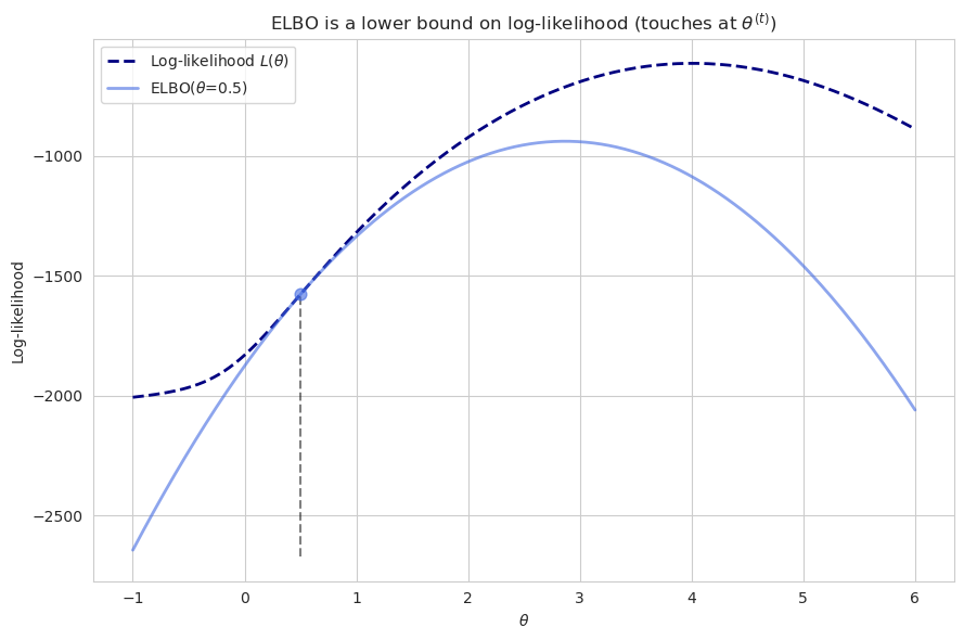

As we can see, at this point this other function is touching the likelihood function but it never outgrows it. This expression is known as Evidence Lower Bound (ELBO).

When $\theta^{(t)}$ is equal to $\theta$ the functions touch. This is because the following expression $\frac{P(X, Z | \theta)}{P (Z | X, \theta^{(t)})}$ becomes a constant, and not a function of $\theta$, and thus Jensen’s inequality becomes equality.

This new equation will be the one which we will have to maximize under the M-step (strictly speaking, a part of it called $Q$-function but more to it later). Using the properties of logarithms it can be rewritten as follows:

\[E_{ Z | X, \theta^{(t)}} \left[\log P(X, Z | \theta)\right] - E_{ Z | X, \theta^{(t)}} \left[\log {P (Z | X, \theta^{(t)})} \right]\]

Remember we now need to find new values of $\theta$, and this variable is not present in the second term of the equation, hence it can be disregarded when doing the search. Therefore, the task of maximizing the log-likelihood boils down to maximizing this:

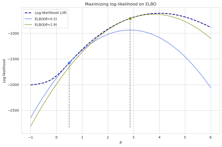
\[Q(\theta | \theta^{(t)}) = E_{ Z | X, \theta^{(t)}} \left[\log P(X, Z | \theta)\right]\]

This final expression is usually relatively easy to solve because $Z$ is obtained by our previous estimate of $\theta$ and $X$. Maximizing it will monotonically increase the true log-likelihood.

Then, after $Q$ is maximized, we obtain updated values of $\theta$, and using them it is possible to construct a new ELBO with new $Q$ function, and then iterate further until the convergence to the local maximum of the true log-likelihood function.

Applications

The EM algorithm is a powerful tool because it turns a hard optimization problem (finding parameters when data is missing) into a sequence of simpler ones. Its general framework can be applied to many different models, including:

• Kalman Filters: The EM algorithm is used to estimate the unknown process and measurement noise covariances ($Q$ and $R$) from time series data. In this case, the latent variables are the true, unobserved states of the system.

• Hidden Markov Models (HMMs): The EM algorithm is used to learn the transition and observation probabilities for a system with hidden states.

• Topic Modeling: Algorithms like Latent Dirichlet Allocation (LDA) use a form of EM to infer the topic mixture of a document and the word distribution of each topic.

In all of these cases, the EM algorithm provides an elegant solution by iteratively refining its beliefs about the unobserved variables and updating the model parameters to best fit those beliefs.