Neural Networks
In this article
- Overview
- Perceptron
- Activation function and learning
- Types of activation functions
- Number of nodes and layers
Overview
Neural network is an algorithm used in machine learning which learns underlying patterns and relationships in the data in a way similar to the neurons in the human brain, hence the name.
The neural networks consist of separate nodes (neurons) which are organized into layers: an input layer, one or more hidden layers, and an output layer. Each node within each layer is connected to every other node in the neighboring layers.
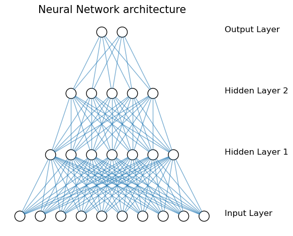
The neural networks which have more than three layers are commonly called deep neural networks.
In the simplest form, the information is passed in one direction only: from the input layer to the output. This is known as feed-forward networks, and in this particular article we deal mostly with them. In the layers which are behind the input layer each node receives information from all nodes of the preceding layer with a certain weight assigned to it. In other words, each nodes gets a linear combination of the features from the previous layer. Then some activation, usually a nonlinear function, is applied to the node, and its result is passed further in the direction of the output layer. Further we shall take a look at what it achieves but first let us see what the network does at the level of a single node. Back to top ↑
Perceptron
The most basic neural network is known as perceptron, and it has just a single node in a single hidden layer.
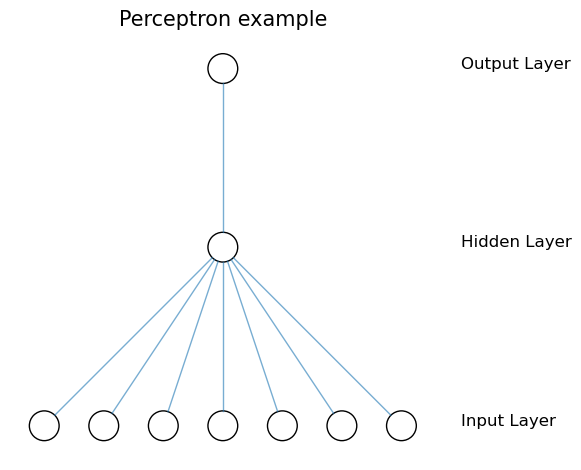
In its hidden layer the perceptron model contains a node which is formed by the linear combination of the input nodes (features) plus bias (or intercept). Then, typically a step activation function is applied to it so that for example the positive values become ones, and the rest - zeros. In fact any threshold value can be used to distinguish the two classes, and it does not need to be zero, but it is commonly expressed as a comparison of a sum of the weighted linear combination and a bias (threshold) which is compared to zero. If the result is greater than zero the neuron is considered to be “fired” or activated.
The perceptron transforms the continuous range into a binary variable, and the input data is separated by a hyperplane into two classes. The step activation function may be substituted by a sigmoid one, and in this case we will get the logistic regression.
If the perceptron model is used for regression task then no activation function is applied, and we simply get the linear regression. Back to top ↑
Activation function and learning
At the level of a single neuron in a hidden layer, the activation function transforms a linear combination of variables into a number which better fits the learning objective. If there are multiple neurons, then each produces its own number using the same activation function but with different weights of the variables from the previous layer. In this way we get a new set of variables corresponding to the number of nodes in the layer, which further can be linearly combined.
The vectorized view of what goes on in the hidden layers of networks can be expressed like this:
\[a^{l} = \sigma(W^l a^{l-1}+b^l) = \sigma(z^l)\]where $a^{l-1}$ is the vector output of a certain layer of the order $(l-1)$, $W^l$ is the weight matrix, $b^l$ is the vector of biases, $z^l$ is the weighted input, and $\sigma$ is the activation function. The number of rows in $W^l$ corresponds to the number of variables in layer $l$, and the number of columns - to the number of variables in the previous layer.
The non-linear activation function transformes the original input space by stretching, squeezing and bending it. In case of classification for instance, different classes become linearly separable in this new transformed space.
In the perceptron example above the step function was used as an activation function. In practice however, if we want to predict more than two classes then the neurons of the output layer should produce the continuous values instead of the binary ones so that we could decide which class prediction is the most likely (which neuron produces the largest number).
The choice of the particular activation function makes an impact on the way the network actually learns because it will have to calculate partial derivatives with respect to each input variable using that particular function. The learning process happens via adjusting of the weights at each node so that the loss function is minimized. The minimum of the loss function is found using the gradient descent where the derivatives determine the scale and direction of the change which should be applied to the input weights in order to reduce the the loss function.
Some additional hyperparameters such as the learning rate, the batch size, and the number of epochs serving as a stopping criterion are selected during the training of the network. Back to top ↑
Backpropagation
In the feed-forward networks the adjustment of the weights is done via an algorithm called backpropagation which sequentially computes the gradients at each node starting from the last layer and going backwards. After learning all the gradient values, the algorithm nudjes all weights and biases simultaneously, making them more optimal with respect to the cost function.
So having in total $L$ layers, it is possible to express the gradient of the loss function with respect to the weights of the last layer using the chain rule:
\[\frac{\partial C}{\partial w^L_{jk}} = \frac{\partial C}{\partial a^L_j} \frac{\partial a^L_j}{\partial z^L_j} \frac{\partial z^L_j}{\partial w^L_{jk}} = \frac{\partial C}{\partial a^L_j} \frac{\partial a^L_j}{\partial z^L_j} a^{L-1}_k\]where $C$ is the cost function (usually the mean squared error), $j$ is an index of a certain node, $k$ is an index of a certain weight which is used in the $j$th node.
Similarly, this is how the gradient with respect to the bias of the last layer is calculated:
\[\frac{\partial C}{\partial b^L_j} = \frac{\partial C}{\partial a^L_j} \frac{\partial a^L_j}{\partial z^L_j} \frac{\partial z^L_j}{\partial b^L_j} = \frac{\partial C}{\partial a^L_j} \frac{\partial a^L_j}{\partial z^L_j} 1\]The common part in both equations is known as the local gradient. We shall write it down once again because it will be used later when moving deeper into other layers:
\[\frac{\partial C}{\partial a^L_j} \frac{\partial a^L_j}{\partial z^L_j} = \delta^L_j\]Now, moving backwards it is possible to calculate sequentially the gradients in the previous layers. But first let’s see how the local gradient of a deeper layer can be expressed using the value of the local gradient of the next layer:
\[\delta^l_j = \frac{\partial C}{\partial z^l_j} = \sum_k \frac{\partial C}{\partial z^{l+1}_k} \frac{\partial z^{l+1}_k}{\partial z^l_j} = \sum_k \frac{\partial z^{l+1}_k}{\partial z^l_j} \delta^{l+1}_k\]In the last part of the equation above the two terms were swapped in the product so that the first element becomes equivalent to the local gradient of the next layer. Regarding the second term note that
\[z^{l+1}_k = \sum_j w^{l+1}_{kj} \sigma(z^l_j) +b^{l+1}_k\]So its derivative with respect to $z^l_j$ is this:
\[\frac{\partial z^{l+1}_k}{\partial z^l_j} = w^{l+1}_{kj} \frac{\partial a^L_j}{\partial z^L_j}\]Then substituting it back into the equation of the local gradient of the $l$the layer it becomes this:
\[\delta^l_j = \sum_k w^{l+1}_{kj} \frac{\partial a^L_j}{\partial z^L_j} \delta^{l+1}_k\]Finally, using this expression one can easily get the gradients of the weights and biases in each further layer. Back to top ↑
Types of activation functions
Let’s look closer at some of the activation functions used in neural networks and see the pros and cons of each.
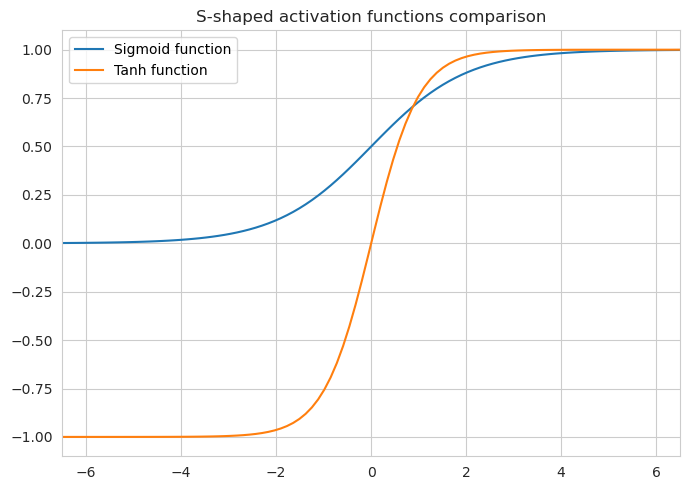
Sigmoid function
As was mentioned previously, this function does transformation just the same way as the logistic regression does by producing a continuous variable which is bounded between 0 and 1. The sigmoid function is expressed like this:
\[\sigma(z) = \frac{1}{1+e^{-z}}\]The benefit of this type of activation function is that it is smooth so the calculation of the gradient should not be an issue. Additionally, the fact that the output is bounded is also a neat property.
And yet, if the input of the function is far away from zero then the gradient becomes so small that it hardly has any impact on the convergence, thus the network learns slowly. This issue is exacerbated by the fact that when calculating the derivatives in the deeper levels one has to multiply by the gradients of the upper levels. So if we get a small gradient value somewhere near the output layer, it will cause an even smaller gradient for the deeper layers. This issue is known as the vanishing gradient.
Additionally, if a certain neuron is close to its optimum, its gradient hardly produces any changes and this is yet another reason why almost nothing is backpropagated to the lower level neurons. This situation is described as a saturated neuron, and it may be an issue if a network recognizes one of its upper layer neurons as saturated during preactivation because it will not contribute anything to the actual learning. Back to top ↑
Tanh function
This one is very similar to the sigmoid function.
\[\sigma(z) = \tanh(z) = \frac{2}{1+e^{-2z}} - 1\]This function is bound between -1 and 1, and it is different from the sigmoid function in that its gradients are somewhat steeper if the input is close to zero. This means that it takes bigger steps near the center of the input space. However, the function still suffers from a problem of the vanishing gradient, just like the sigmoid function.
 Back to top ↑
ReLU
Rectified linear unit or ReLU is usually a default option for activations when building and testing neural networks. It is expressed like this:
\[\sigma(z) = \max(0, z)\]Although it looks like a piecewise linear function it is considered to be non-linear. At the level of a single layer of a network a linear combination of linear functions is still a linear function. A linear combination of ReLU functions however can model complicated shapes fairly well.
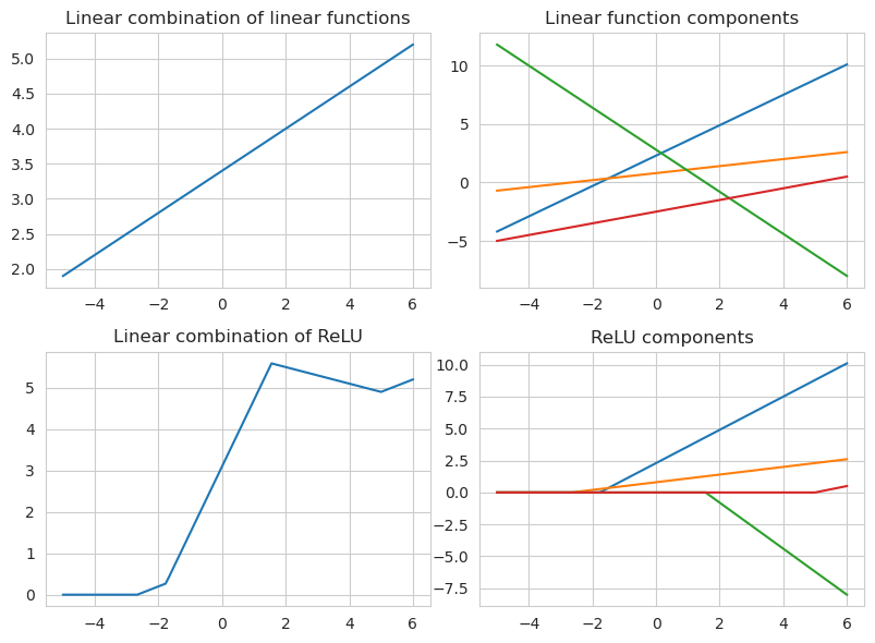
ReLU has an advantage over other activation functions in that it is much more efficient in terms of optimizing the loss function via the gradient descent. It never saturates on plateau like the sigmoid and tanh functions do. If the input of the function is a positive number then the derivative of $z$ is 1, and if the output is negative then the derivative is equal to 0. The sparsity of the network is generally good because it simplifies the model and lets it learn only the meaningful features while also making it faster.
On the other hand, the zero derivative output in certain neurons does not backpropagate anything (because of multiplying by 0), and thus the neurons of the deeper layers aren’t learning anything. If the learning rate is too high or if the network learns a big negative bias from its weights, a neuron becomes stuck with the negative inputs, it will always produce zeros, and this leads to so-called dying ReLU problem.
One of the suggested ways to combat the dying ReLU issue is to output $0.01x$ instead of 0 when the input of the function is negative (leaky ReLU). In this way the learning will be enabled. Another alternative, namely parametric ReLU, is to make the network learn a special parameter $\alpha$ for each layer which is used instead of 0.01 of the leaky ReLU.
Another disadvantage of ReLU is that due to the positive gradient the values of the weights of the connected nodes can only move in one direction during an update. Let’s take a look at the equation of the gradient of the weights again:
\[\frac{\partial C}{\partial a^L_j} \frac{\partial a^L_j}{\partial z^L_j} a^{L-1}_k\]The first multiplier can be either positive or negative depending on whether the predicted output is bigger or smaller than the actual observation. The second one is just 1 (if the neuron is not dead). If the activation function at the previous layer is also ReLU then the third multiplier is either positive or zero. This means that in each epoch the adjustment of all of the weights of the non-dead nodes will be nudged in the same direction: either positive or negative, which might not be optimal. Back to top ↑
ELU
Exponential linear unit or ELU is a proposed improvement over ReLU which is albeit more computationally intensive, outperforms it in terms of convergence rate and neural network prediction accuracy. The idea of ELU is to continue the function nonlinearly for the negative inputs, and saturate it at a certain level.
\[\sigma(z) = \Bigg \{ \begin{array}{ll} z &\text{if } z > 0\\ \alpha (e^z - 1) &\text{if } z \leq 0 \end{array}\]Here $\alpha$ is a hyperparameter which is usually set as 1 in practice, although it can assume values between 0 and 1.

ELU has the advantage of ReLU of the efficient gradient calculation if the input of the node is positive, and at the same time it prevents the dying of the nodes by allowing them to assume negative values. Unlike the leaking and parametric RelU, ELU does not have the point of discontinuity near 0. It also bounds the negative output at a certain level so that it doesn’t become too big and prevents other nodes from being positive. Back to top ↑
Softmax
This activation function is generally used in the output layer for multiclass classification.
\[\sigma(z_i) = \frac{e^{z_i}}{\sum_{j=1}^K e^{z_j}}\]The function takes a vector $z$ consisting of $k$ elements and outputs the vector of probabilities proportional to their exponentials. Applying exponential takes care of the negative and zero output values. Back to top ↑
Number of nodes and layers
As you may guess by now, in neural networks the number of nodes in the input layer equals the number of features of a model. The number of output nodes usually equals the possible number of predicted classes unless we are dealing with a binary classification where it would be sufficient to have only one output node. In regression models there is only one output node as well. The number of nodes in each hidden layer is usually smaller than in the previous layer, and is generally better determined via experimentation. As for the number of layers - the more the better; however at a certain point adding an additional layer would not lead to the improvement of the model but make computation more expensive so one should experiment with this hyperparameter as well. Back to top ↑