Outliers detection
This article explores machine learning models used to identify unusual or atypical observations within data sets.
A crucial distinction should be made based on the properties of the training data.
-
Outliers detection (unsupervised learning). When the training data likely contains atypical observations, or the data’s characteristics are unknown, outlier detection is employed. This is an unsupervised machine learning task, meaning the model doesn’t rely on pre-labeled data for atypical examples. Here, unusual observations typically reside in areas of low data density.
-
Novelty detection (semi-supervised learning): Conversely, when the training data is known to be free of atypical observations, and the goal is to identify potential anomalies in new data, novelty detection is used. This is a form of semi-supervised learning, as the model leverages labeled data (clean observations) for training and unlabeled data (new observations) for anomaly detection. In this scenario, atypical observations can form new high-density regions; they simply need to deviate from the established group of observations.
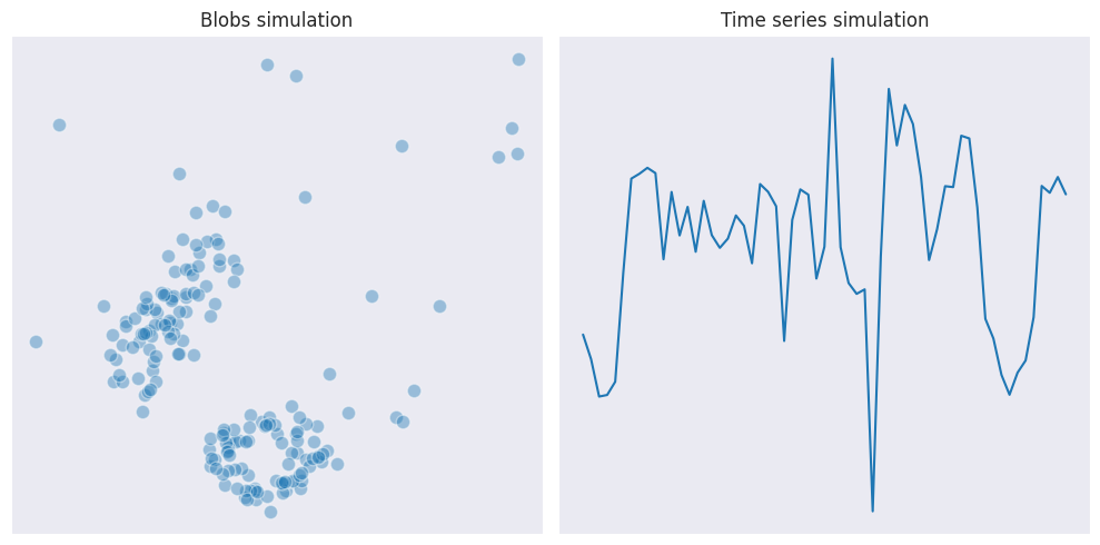
We will consider several algorithms used for outlier detection using these simulated data samples:
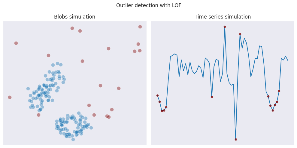
Local outlier factor (LOF)
This is a density-based technique of identifying outliers where the local density is measured at each data point and then compared with the average density in the local region. If it’s significantly lover - then it is an outlier.
The local density is defined using the data from $k$ nearest neighbors with respect to the given point. This has an advantage of comparing only against the nearest cluster of points instead of the whole dataset where the values may vary significantly.
For each point LOF determines its core distance (or radius) - the distance to the $k$th nearest neighbor, and the reachability distance from each of its $k$ neighbors. The reachability of $A$ with respect to $B$ is defined as the maximum between the direct distance between the points, and the core distance of $B$.
\[r_{AB} = \max[d_{B}, d(A, B)]\]If $A$ lies within the radius of $B$ then the reachability to $A$ is simply the core distance of $B$, and only if the distance from $A$ to $B$ exceeds the core distance of $B$ ($A$ is outside the radius of $B$) then the reachability to $A$ is the direct distance between $A$ and $B$. This has the effect that all closely lying points within the radius of $B$ have the same reachability from $B$ ($B$ does not view them as outliers, they are “reachable” for the given value of $k$, so treated equally). In practice this makes the algorithm more robust.
Then the local reachability density of $A$ is defined as an inverse of the average reachability distance to it among all potential points $B$ in its neighborhood:
\[lrd_{k}(A) = \frac{\lvert N_{k}(A) \rvert}{\sum_{B \in N_{k}(A)} r_{AB}}\]Inverse is used because bigger distances lead to the decrease in density and vice versa.
The local outlier factor for $A$ is the normalized version of the local reachability density which is calculated as the average ratio between $lrd_{k}(A)$ and $lrd_{k}(A)$ for all $B$ which are in the neighborhood of $A$:
\[LOF_{k}(A) = \frac{\sum_{B \in N_{k}(A)} \frac{lrd_{k}(B)}{lrd_{k}(A)}}{\lvert N_{k}(A) \rvert}\]If the resulting metric is close to 1 then the local density around $A$ is similar to the density at its neighbors. If it is bigger than 1 then there are chances that $A$ is an outlier.
Here is how the algorithm performs on our test data:
GLOSH
Global-Local Outlier Score from Hierarchies (or simply GLOSH) builds upon a clustering method called HDBSCAN to identify outliers.
Since according to HDBSCAN the points are grouped into clusters according to their density, the local outliers are then identified by comparing a data point’s density with the density of its cluster. Similarly to LOF, GLOSH calculates a score for each data point, which reflects how much the point’s density deviates from the density of its cluster.
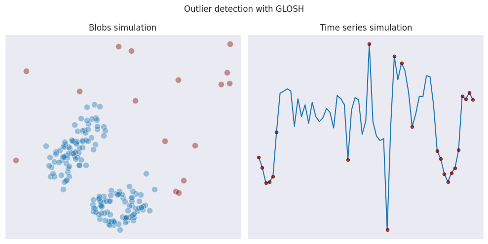
Compared to LOF, in our example GLOSH marks more points as outliers in case of time series simulation because it considers the first and the last points as being far away from the clusters in the middle. THis is a reason why GLOSH is less suited for detection of anomalies in time-series data.
In case of blobs data, GLOSH seems to be less strict when determining outliers, allowing points being associated with certain clusters.
Isolation forest
This an algorithm which is similar to the random forest in a way it creates trees and performs splits but which is more geared towards detection of outliers.
Each tree selects a random subset of data, then randomly selects a feature, and performs a random split between its maximum and minimum values. Then the splitting is performed further until all data points are isolated or when the maximum predefined depth of the tree is reached.
Since outliers are inherently different from the bulk of the data, they’ll tend to be separated by the random splits much earlier in the tree building process compared to points within dense clusters. This translates to a shorter “isolation path length” for outliers.
The algorithm uses the average path length across all trees to determine an anomaly score of each data point.
Isolation forest has good properties in terms of scalability, as it creates subsamples of data. It also can be used for novelty detection.
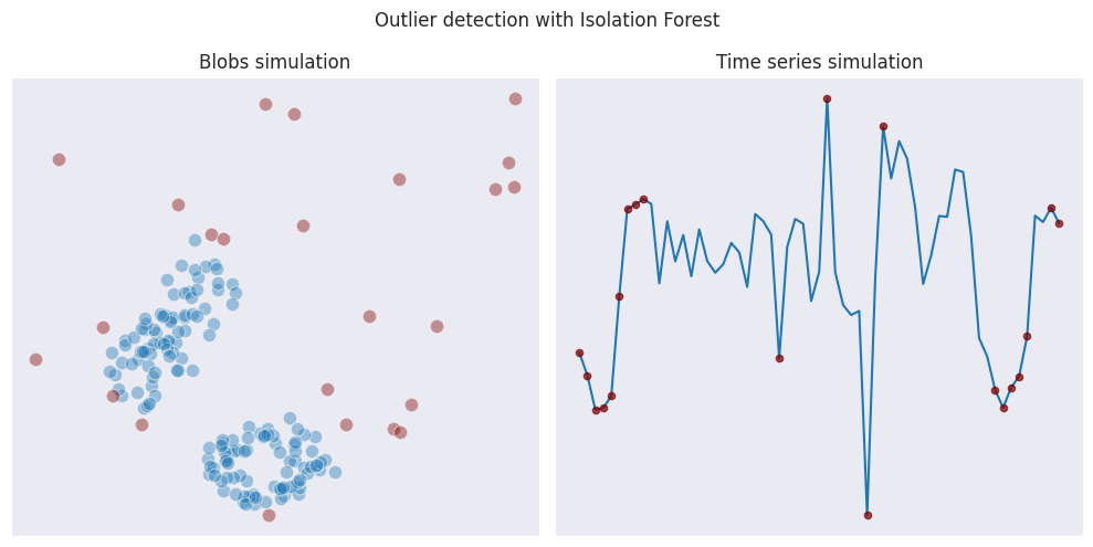
Similarly to GLOSH, Isolation forest suffers from the same issues when determining outliers on the edges of time series data. When dealing with blobs data, its behavior is more aggressive than GLOSH and LOF.
Choosing the right model for outlier detection
There’s no one-size-fits-all solution for outlier detection. Different models excel in various scenarios. To determine the best fit for your data, evaluate several models on a representative subset. The described models assign scores to data points so one can adjust the threshold used to classify points as outliers based on specific needs.
Granted, not all datasets have only two dimensions, so it might not be possible to visualize the results. Dimensionality reduction techniques, such as principal component analysis, can project high-dimensional data onto a two-dimensional plane, enabling visualization.
If there is prior knowledge about the true outliers from the dataset then it is possible to build a confusion matrix, calculate ROC curves, and compare the performance in this way.