Clustering overview

21 minute read

Clustering may be viewed as grouping of data points according to their similarity so that the most similar points end up being in the same cluster. Clustering has wide practical application, including customers and products segmentation, and detection of anomalies. There are numerous models which can be used for clustering. Primarily they differentiate by how they determine the level of similarity between data points, while also they can rely on other conditions, such as enforcing only some fixed number of clusters and allowing data points to not belong to any cluster.

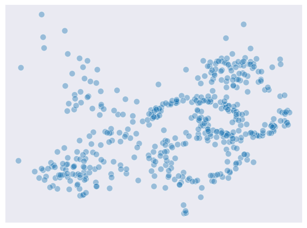
Will will test several prominent clustering algorithms on the 2-dimensional dataset visualized below. This dataset clearly has the regions of high density with several interconnected areas which leaves some ambiguity.

K-means

This is the most simple clustering model which can be used as a benchmark when comparing performance of other ones. Under K-means the number of clusters should be provided beforehand so that the points could be distributed among $n$ groups. The distribution is done by minimizing the sum of inner variance within each cluster (also called inertia).

\[\sum_{i=1}^n (\lvert\lvert x_i - \mu_j \rvert\rvert^2)\]

where $\mu_j$ is the centroid of $j$th cluster.

The initialization of the algorithm is done by specifying centeroids - they might be selected as some of the existing points in the dataset but can be really any random points in the dataspace. Each sample is assigned to the nearest centroid, and then new centroids are recalculated as the mean values over each of the formed clusters. Then the process is repeated a number of times until the change in centroid values becomes small enough.

The choice of initial centroids is important as the algorithm may converge to some local optimum. Other than that, K-means performs poorly if the clusters have elongated or folded shapes.

K-means++

This is an improvement over the standard algorithm whereas the initial points are selected automatically and not at fully at random. The idea behind this approach is that the initial points should be spread from each other at maximum. Here is how it proceeds:

First cluster centroid is selected randomly uniformly from the data.
For each data point which remains, the distance is computed between it and the nearest center that has already been chosen.
A new data point is chosen randomly as a new center using weighted probability distribution built from to the squared distances.
Steps 2 and 3 are repeated until K centers are chosen.

Let’s see how the algorithm performs on our testing dataset.

The results are not too bad but neither are impressive because the algorithm simply divided the whole dataset into 6 parts without considering internal structure. This is why the moon-shaped clusters are split into different ones according to K-means. We will keep this result as a benchmark to compare against other potentially better algorithms.

Mini-batch K-means

This version of the algorithm is aimed at improving the speed of computation albeit the correctness of the output might be lower. The idea is similar to that of the mini-batch gradient descent: the samples are drawn randomly from the whole dataset, and for each sample in the mini-batch, the assigned centroid is updated by taking the streaming average of the sample and all previous samples assigned to that centroid. Back to top ↑

Hierarchical clustering

These models can be divided into two groups: agglomerative and divisive. The former start off by considering each single datapoint as a separate cluster and then merge them into bigger ones until a single cluster is formed. The latter start off with a single cluster and then divide it into smaller one.

In exploratory data analysis dendrograms are used for visual representation of the linkage between clusters, so that the number of clusters may be deduced.

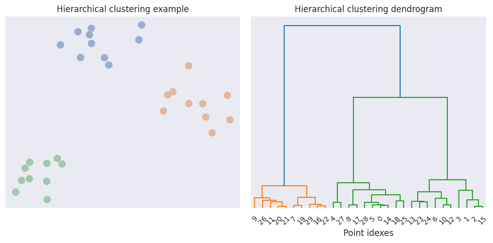
The dendrogram displays connections between the initial data points and newly formed clusters. The vertical lines indicate which points and clusters are being merged, and the height of the upper link indicates the distance between them. From the example above we can see that the distance between clusters in the last two merges is significantly larger than the distances of the previous merges, therefore we may reasonably assume that there are 3 clusters in total.

Before merging clusters in the agglomerative type of clustering some measure of distance should be evaluated in order to determine which ones are the closest ones, so that they can be merged together. The distance may be calculated using different type of linkage:

single linkage - where the distance between clusters is the shortest possible distance between the points belonging to each of the two clusters.
maximum (or complete) linkage - where the distance is the biggest possible distance between the points of two clusters.
average linkage - where the distance is the average distance of every point in the cluster with every point in another cluster.

Other than that, ward linkage may be used which determines clusters by minimizing the sum of squared distances (sum of squared errors or SSE) when merging smaller clusters into bigger ones. According to this method, the within-group sum of distances is considered, similarly to K-means. Unlike K-means however the members of the already formed clusters do not come and go if the centroid changes - they were already included during previous iterations of merging.

For example we have clusters A and B with their own within-group distances.

\[SSE_{A} = \sum_{i=1}^{n_A} (\lvert\lvert x_i - \mu_A \rvert\rvert^2)\] \[SSE_{B} = \sum_{i=1}^{n_B} (\lvert\lvert x_i - \mu_B \rvert\rvert^2)\]

Supposing we merge these two clusters then it is possible to calculate the between group sum of squared errors with respect to the new central point of the newly merged cluster.

\[SSE_{AB} = \sum_{i=1}^{n_{AB}} (\lvert\lvert x_i - \mu_{AB} \rvert\rvert^2)\]

When determining which two clusters to merge, the ward linkage is guided by the following minimization criteria:

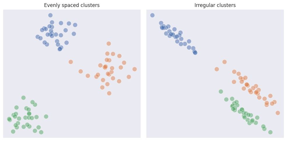
\[I_{AB} = SSE_{AB} - (SSE_{A} + SSE_{B})\]

Compared to K-means, ward linkage in agglomerative clustering has a better grasp on the structure of clusters producing more accurate results. Compared to the single linkage, ward expects clusters to be more evenly spaced which may not always be the case, especially if the shapes of the clusters are irregular. On the other hand, single linkage may fail if it is expected for clusters to be round and somewhat evenly spaced because outliers may lead to classifying them as separate clusters.

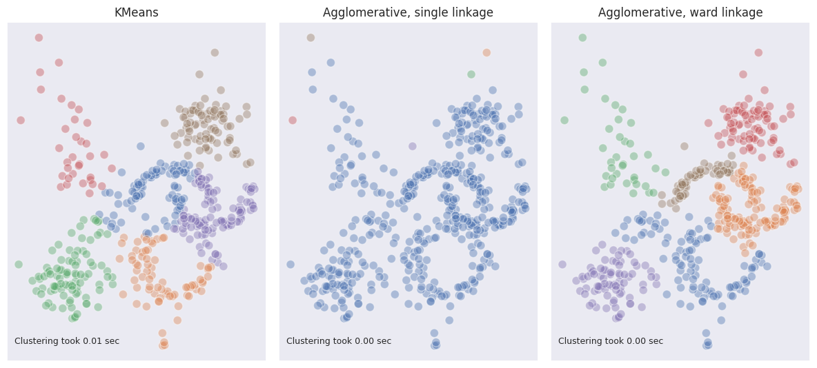
From the example above we see how single linkage fully fails in case of multiple dense regions and outliers. Ward linkage however outperformed K-means in terms of visual matching.

BIRCH

BIRCH stands for Balanced Iterative Reducing and Clustering using Hierarchies. This algorithm can be used as an intermediate step to other clustering algorithms because it transforms the data points into subclusters by grouping them into blobs. After that any other clustering algorithm can be applied to these initial subclusters.

BIRCH builds clustering feature tree (CFT) which have nodes, which in turn may have their own nodes as children. Each node in this tree is a subcluster with its own coordinates and centroid.

In the scope of BIRCH the raw data points are processed one by one. They go through the root of the CFT and are assigned to a node of a subcluster which will have the smallest radius after adding this new data point. If the subcluster has any child node, then this new point is passed further down repeatedly until it reaches the lowest level subcluster - a leaf. After adding, the properties of each subcluster are updated.

Each of the lowest level subclusters have their own threshold value which defines its radius. If after adding a new datapoint the radius exceeds the threshold, then a new subcluster is formed horizontally, and the points are redistributed between the existing nodes.

Additionally the trees have a so-called branching factor which restricts the number of nodes from the same parent node. If after branching the number of subclusters starts exceeding the branching factor then the parent node is split.

Eventually any clustering algorithm is applied to the leaf-level subclusters of CFT. Here is the result of BIRCH followed by agglomerative clustering with ward linkage compared to agglomerative clustering without BIRCH.

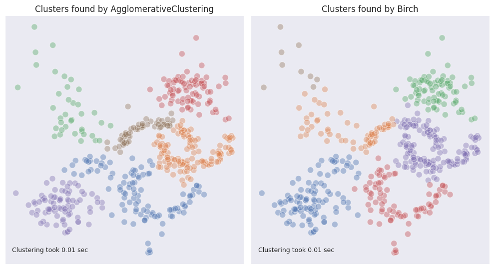
As can be seen, BIRCH performed worse here because it merged clusters with varying densities together.

Affinity propagation

According to this algorithm the dataset can be explained by a small set of exemplars - the observations which correspond to clusters of data. The algorithm identifies clusters by iteratively sending messages between data points to determine which points should be considered as exemplars.

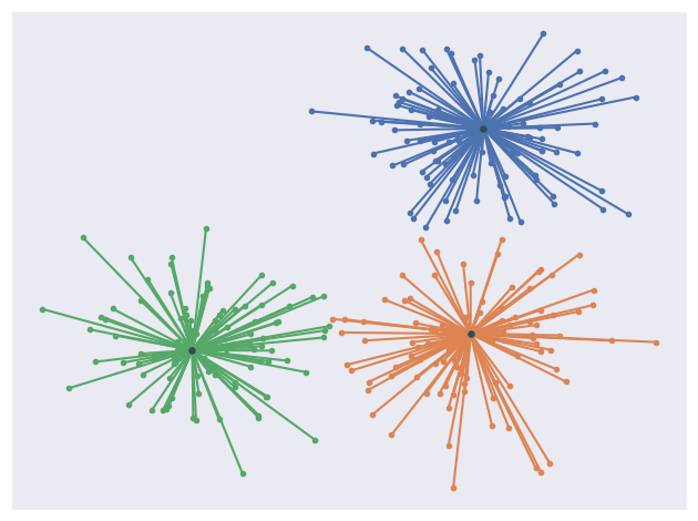
The greatest benefit of Affinity propagation is that it determines the number of clusters automatically.

The algorithm begins with a similarity matrix $S(i, k)$, where each element represents the similarity between pairs of data points. The similarity can be measured using the negative Euclidean distance.

The diagonal elements are overwritten to be a certain number called “preference”. This number works as a parameter which has an impact on the resulting number of classes: the closer the number to the maximum similarity among individual data points - the more classes will the algorithm produce. Typically preference is set to be a median of the calculated similarities. It might seem counterintuitive but in fact this serves a purpose of preventing the data points to select themselves as the exemplars.

Other than that, matrices of responsibility and availability are initialized at zeroes and updated at each iteration. Responsibility matrix $R(i, k)$ contains information about how well-suited $i$ finds data point $k$ to become its exemplar. A high value indicates that a data point is a good candidate to be an exemplar.

Availability matrix $A(i, k)$ contains information about how appropriate it would be for $k$ to represent $i$ as its exemplar. It reflects the accumulated evidence from other points nominating it as an exemplar.

Let us consider how the individual elements of the matrices are updated. First the responsibility updates are calculated:

\[r(i, k) \leftarrow s(i, k) - \max [ a(i, k') + s(i, k') \forall k' \neq k ]\]

When determining the responsibility of $k$, each $i$ checks the maximum sum of similarity and availability among all other potential exemplars with respect to itself. Then it compares its similarity $s(i, k)$ with potentially best other exemplar. The resulting positive responsibilities are good candidates because their similarity measure is higher than that of any other data point.

Next step is updating the availability matrix:

\[a(k, k) = \sum_{i' \neq k} \max[0, r(i', k)]\] \[a(i, k) \leftarrow min [0, r(k, k) + \sum_{i' \notin \{i, k\}} \max [0,{r(i', k)}])]\]

The availability of $k$ to be an exemplar for itself is simply the sum of all positive responsibilities which other data points deem for $k$. The availability of $k$ for $i$ similarly depends on the sum of other points’ positive responsibilities deemed for $k$, plus the responsibility which $k$ puts on itself (its willingness to be its own exemplar) which could be negative. The resulting value is capped at zero in order to balance the convergence. As can be seen, the non-diagonal elements of $A(i, k)$ are either negative or zero.

The unwillingness of $k$ to be its own exemplar can cancel out the fact that other data points view it as a good exemplar for themselves and thus the number of clusters eventually is less than the number of datapoints: this is the effect of putting the “preference” parameter in advance.

The final exemplars are determined after either convergence or exhaustion of the number of iterations. They are taken from the elements where the sum of responsibility and availability is positive.

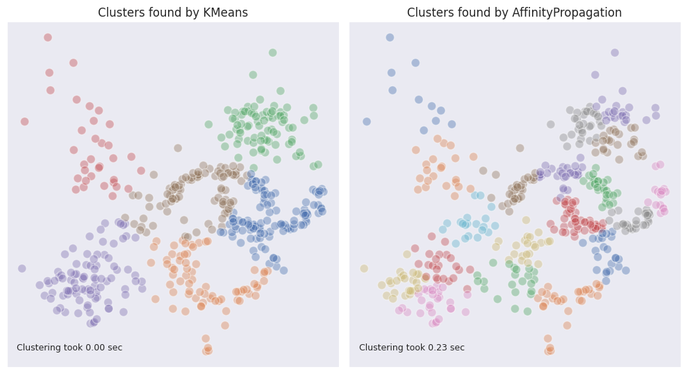
One of the drawbacks of this method compared with the others is its complexity. Additionally, the affinity propagation algorithm will not typically produce the best results of clustering. As can be seen below, in our example dataset it produces too many clusters if the preference is not specified. The increase in time is also considerable.

Mean shift

Mean shift clustering is a non-parametric clustering algorithm that doesn’t require specifying the number of clusters beforehand. It achieves this by dynamically identifying clusters based on the density of data points in the feature space.

In the scope of this algorithm, at the beginning each data point is considered as a cluster center. Mean shift uses a kernel function, typically a Gaussian kernel, to measure the similarity between data points. This kernel function determines the influence of nearby points on the current point. Then for each data point, it iteratively shifts its cluster center towards the mode (peak) of the data distribution within a certain neighborhood, until convergence. The shift is determined by computing the mean of the points within the neighborhood, weighted by the kernel function.

The main drawback of Mean shift is that it is computationally expensive, as it requires calculating distances between all pairs of data points in each iteration. At the same time, the benefit of not specifying the number of clusters is canceled out by the necessity to specify the bandwidth parameter, otherwise the result of clustering won’t be satisfactory.

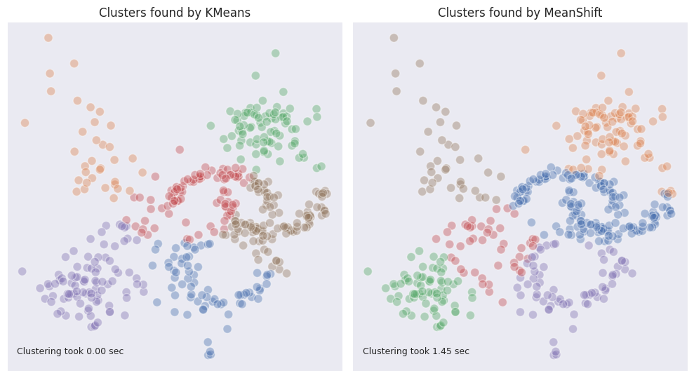
The output of Mean shift for our example dataset looks quite well, yet it was achieved by careful fine-tuning of the bandwidth parameter. In real life situations the dimensionality of data is higher than two so the bandwidth will not be possible to select empirically.

Spectral clustering

This algorithm considers a dataset as a graph of interconnected points $G(V, E)$, where $V$ are vertices (or nodes) and $E$ are edges connecting the vertices. The edges between nodes represent the similarity between the corresponding data points. This similarity is typically computed using a Gaussian kernel or some other similarity measure.

The clusters are found in such a way that they represent regions where the graph has many crossings $E$ while the interconnecting regions have only few of those.

A square symmetric adjacency matrix $A$ is constructed for each node where each of the crossings of the rows and columns reflects whether the nodes are connected. If the nodes are connected then the corresponding element of $A$ is 1, otherwise 0, including its diagonal elements.

In addition to the adjacency matrix, a degree matrix $D$ is defined, which is a square diagonal matrix whose values represent the number of connections each node has which is called the degree. Then a Laplacian matrix is constructed as $L=D-A$ which encompasses the complete information from the graph.

According to the graph theory, the “spectrum” of the graph $G$ is the set of eigenvectors of the any matrix (Laplacian or adjacency matrix) ordered by their eigenvalues. For instance, the Laplacian matrix has useful properties such as its eigenvectors are real and orthogonal, and the eigenvalues are non-negative numbers. Another interesting property is that the sum of each row is equal to 0 (because from the number of connections each of them is subtracted).

In scope of the Spectral clustering the Laplacian matrix is decomposed into eigenvectors and eigenvalues. These eigenvectors form a new space in which the data points are embedded.

The smallest eigenvalue of $L$ is always zero, and the corresponding eigenvector contains ones. This is due to the fact that multiplication of Laplacian with the vector of ones produces a vector of zeros, and it is the same result which would have been obtained when the vector of ones is multiplied by zero- a fundamental property of eigenvectors and eigenvalues.

The top $k$ eigenvectors corresponding to the smallest eigenvalues are typically selected (excluding the first eigenvector, whose eigenvalue is zero) - they correspond to the basis dimensions along which the variance is the lowest, in case of the Laplacian matrix - to the weakly connected regions of the graph $G$.

In the reduced-dimensional space, traditional clustering techniques like K-means are applied to cluster the data points, and finally, the cluster labels assigned by the clustering algorithm are propagated back to the original data points.

A more advanced technique in spectral clustering is the usage of QR factorization over the eigenvector matrix which is obtained from the adjacency matrix. Through a series of orthogonal transformations $X$ starts resembling the indicator matrix $W$ of size $n \times k$. The rows of $W$ represent observations while its columns represent clusters. The elements of $W$ are either 1 if the observation belongs to a particular cluster, or 0.

On our example dataset the spectral clustering achieved a comparable result with that of the agglomerative clustering with ward linkage.

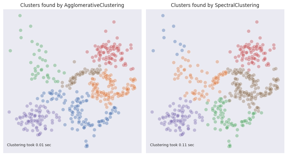
In some ways it performed better, for example it was able to separate the points on the left from the circle. At the same time it included a part of the moon-shaped figure into a cloud of points, which is not desirable.

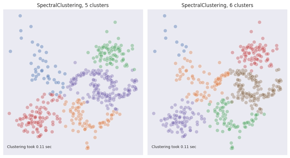
When tinkering with the number of clusters, it was observed that the algorithm performed much better when it was set to 5 instead of 6, but again, this is not what is usually known in advance.

DBSCAN

DBSCAN stands for Density-Based Spatial Clustering of Applications with Noise. DBSCAN operates based on the idea that clusters are dense regions of data points separated by regions of lower density.

DBSCAN defines two key parameters: the radius of the neighborhood around each data point $\varepsilon$, and the minimum number of points required to form a dense region or cluster. Based on these parameters, it categorizes data points into three types:

Core Points. A data point is considered a core point if it has the required minimum of other points within its radius.
Border Points. A data point is considered a border point if it’s not a core point but lies within the radius of a core point.
Noise Points (Outliers). Data points that are neither core points nor border points.

The algorithm begins by randomly selecting a data point that has not been visited. It then explores its neighborhood to identify all reachable points (core and border points). If the number of reachable points is sufficient then a cluster is formed. For all of the points which are core points within the newly formed cluster the same procedure is done again, and thus other points can be added to the cluster.

DBSCAN is capable of identifying clusters of arbitrary shapes because it doesn’t assume any particular shape for the clusters. It adapts to the local density of the data and forms clusters accordingly. The added benefit is the ability to identify outliers.

The drawback of DBSCAN is that its effectiveness highly depends on selecting the appropriate hyperparameter which corresponds to the radius of the neighborhood. If misconfigured, it can treat the whole dataset as a single cluster, or not find any clusters at all. In this sense even though there is no need to specify the number of clusters, the algorithm needs hyperparameter tuning just like Affinity propagation and Mean shift.

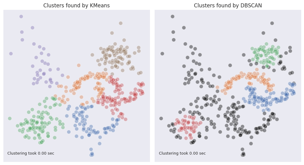
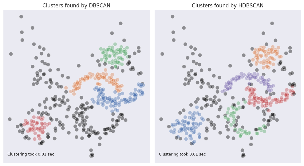
As can be seen, DBSCAN under is capable of identifying moon-shaped clusters fairly well. However, other clusters which have more sparse structure are not so well defined. We can observe that the whole cloud in the top left corner was not labeled. The edges of the two blobs in the top tight and bottom left corners, where the density is lower, were also marked as outliers.

OPTICS

The Ordering Points To Identify the Clustering Structure (OPTICS) algorithm is a density-based clustering algorithm that can be viewed as a generalization of DBSCAN. It attempts to remove the necessity to specify the radius of the neighborhood $\varepsilon$ thus making the algorithm more adaptable to clusters with varying densities. At the same time the requirement to specify the minimum number of points to constitute a cluster remains.

OPTICS starts with a random point, then goes to its nearest neighbor and measures the distance to it. The order and the distance are recorded, after which it moves on the point which is nearest to the second one excluding the already visited one. The process repeates until all points are visited. Eventually, two arrays are produced: the one with the orders of the points, and the one with the distances which were covered from one point to another.

OPTICS builds a reachability plot, where the order is put on the x-axis, and the distance on the y-axis like so:

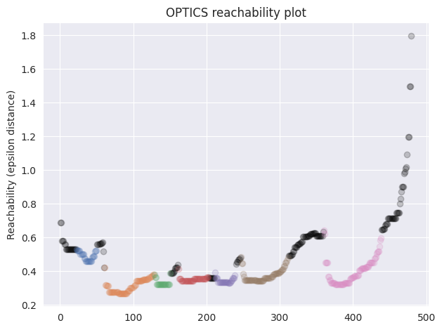
The points belonging to clusters are marked with color while the points which are considered as outliers are black. Intuitively, the decrease in distance means that the algorithm has reached a region of higher density which is why it starts to consider the points as belonging to a cluster, and coloring them accordingly. We can also observe that when the distance starts to increase significantly then the points are no longer considered to be belonging to a cluster, and start marking as outliers instead. Also the clusters with higher density have lower values of reachability.

See the results of OPTICS clustering compared to DBSCAN:

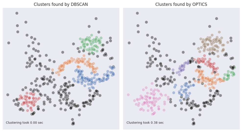
The blob-shaped clusters are better identifiable, and the cloud of outliers is smaller on their edges. At the same time the moon-shaped clusters are split in twos. If we look at the reachability plot we can still observe that the halves are close together, and were split due to the sharp change in density due to the outliers presence. Overall, it may seem like DBSCAN deals better with the clusters of non-standard shape however OPTICS excels in identifying round blobs of varying density while also doing a decent job in identifying clusters of non-standard shape.

HDBSCAN

This is yet another improvement over DBSCAN (H stands for hierarchical) which drops the requirement to specify the radius of the neighborhood $\varepsilon$. Instead, one only needs to specify the minimum number of samples which can constitute a cluster.

Similarly to DBSCAN, HDBSCAN utilizes the idea of core points which form clusters of other points around them. It is possible to specify the number of points in the neighborhood needed for a core point to be considered as such, and this number can be set different from the minimum size of a cluster. Setting it lower than the minimum cluster size will eventually enable detection of clusters with non-standard shapes.

For each point the core distance $d_{c}$ is defined as the minimum radius required in order to have the minimum number of samples in the neighborhood of this sample.

HDBSCAN uses the idea of single linkage from agglomerative clustering in order to merge individual points into clusters. As we know, the outliers have a negative effect on single linkage because they lead to merging of distinct clusters if an outlier happens to be between them. Therefore, in order to dampen the effect of outliers, and to avoid situations when regions with different density are merged into a cluster, HDBSCAN transforms the regions with lower density by making them more distant from regions with higher density. This is done by introducing mutual reachability distance for each pair of points:

\[d_{reach}(a, b) = \max [d_{c}(a), d_{c}(b), d(a,b)]\]

If the distance between points $a$ and $b$ is greater than the core distance of both $a$ and $b$ then it is set as the reachability for these points. If however it is less than the core distance of any of the two points then the largest of the two is selected. In practice it increases the distance thus making the clusters more separable from one another and from the outliers. The points within the radius of a core point are either pushed to its periphery (if they are part of the tightly packed cluster) or outside of it (if they are part of another cluster with lower density or an outlier).

HDBSCAN constructs a graph network where each data point is a node, and the edges are the reachability distances between the points: at this stage all points form a single cluster. Then it starts cutting through the edges starting from the one with the highest distance. Then the distance at which the next cut is performed is selected as the next biggest one, ans so on.

Consequently, the graph is split into smaller and smaller clusters up to the point where the condition of minimum cluster size is reached. However, this is not the final result of the clustering because some of the resulting clusters are better be merged instead of having the number of datapoints near the possible minimum. Therefore, HDBSCAN assesses the persistence of the resulting clusters. It records the number of datapoints in the remaining clusters, the distances at which the next cuts would have been performed if not for the condition of the minimum cluster size, and information about their parent clusters.

These distances are used to construct an auxiliary metric $\lambda$ for each data point within these clusters. It is simply a reciprocal number of the distance at which the point would have been cut out from the cluster, so the bigger the distance - the lower $\lambda$.

Each cluster has its own $\lambda$ of birth and death: the point in time when a cluster was separated from the remaining graph nodes, and the point in time when the cluster was further split into smaller clusters. These metrics are obtained from the distances at which the cut is performed during the described events. It is reasonable to say that $\lambda_{birth}$ is always smaller than $\lambda_{death}$. The points within each cluster have values of $\lambda$ somewhere between $\lambda_{birth}$ and $\lambda_{death}$ for this particular cluster.

HDBSCAN employs an additional metric called stability which is calculated for each cluster like this:

\[\sum_{p}(\lambda_p - \lambda_{birth})\]

where $p$ is a point within a cluster.

The clusters where the points are more tightly packed, have higher stability scores because their $\lambda_p$ are higher (while the distance at which the cut is performed is lower). If the sum of stability of two child clusters is less than the stability of their parent cluster then they are merged together, and thus more persistent clusters are obtained.

As can be seen from the example used in this article, HDBSCAN outperforms DBSCAN and OPTICS.

Share on

Twitter Facebook LinkedIn

Clustering overview

In this article