Logistic regression

Logistic regression is one of the simplests algorithms for binary classification, and it is based on the linear regression. In its core, it uses a linear combination of independent variables which is then transformed into a probability measure using logistic function. Therefore, the output becomes bounded between 0 and 1.

Logistic function

Let’s take a look at the behavior of the logistic function. Its formula is this:

\[f(t) = \frac{e^{t}}{e^{t}+1} = \frac{1}{1+e^{-t}}\]

And it looks like this:

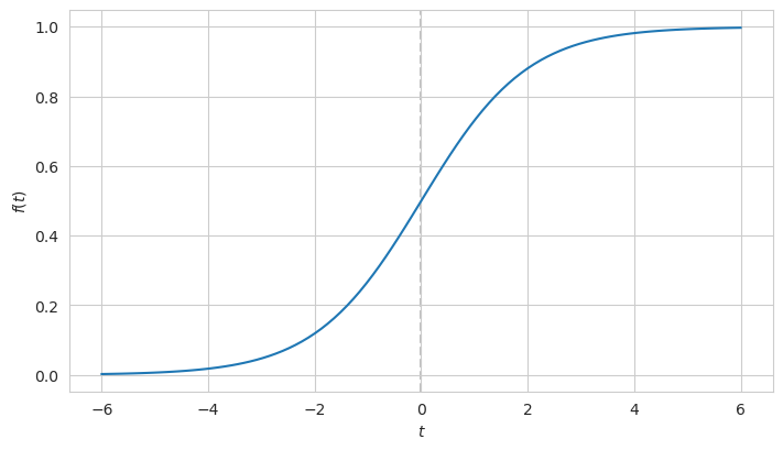
This function assumes values between 0 and 1 but without ever reaching them.

In terms of the logistic regression $t$ is the linear combination of independent variables which is transformed into the probability measure. This linear combination is also equal to the log-odds, that is the logarithm of the ratio between the number of successes to the number of failures, hence the name of the regression.

\[t = \ln \left( \frac{p(y=1)}{p(y=0)} \right)\]

After the parameters of the independent variables are estimated, the fitted line is supposed to separate the two classes of observations using the sigmoid curve.

Goodness of fit

The goodness of fit is optimized by maximizing the likelihood function:

\[\mathcal {L} = \prod_{k:y_{k}=1}p_{k} \prod_{k:y_{k}=0}(1- p_{k})\]

where $y_{k}=1$ and $y_{k}=0$ are observations of success and failure accordingly, and $p_k$ is the estimated probability of success.

For better properties when calculating the derivative, the product is transformed into sum by taking the logarithm of the expression:

\[\ln (\mathcal {L}) = \sum_{k:y_{k}=1} \ln (p_{k}) + \sum_{k:y_{k}=0} \ln(1- p_{k})\]

Making predictions

Usually the predicted probability higher than 0.5 is treated as a success in binary output values, however the threshold can be adjusted to better suit the needs of the case. In certain applications, for example in determining the fraud transactions, it may be critical to reduce the recall metric (the number of false negative) predictions, and thus the threshold may be set lower than 0.5. This will eventually increase the number of false positive predictions but the cost of these errors is far less in this particular situation.

On the other hand, we might want to decide which customers should be granted an additional discount in order to improve their retention. In this case setting the threshold higher than 0.5 may lead to the situation where the discount is not overly spent at cost of some potential loyal customers missed. In this situation the operational revenue won’t be reduced that much but a fraction of the customers may become loyal which would give long-term benefits.

Multinomial classification

Although the logistic regression was designed to tackle the binary classification issues, it can be extended to deal with multinomial cases as well. If there are $K$ distinct independent categories, then it is possible to build $(K-1)$ pairwise models, where one category is selected as a pivot option, and the rest are compared to this one using the log odd like this:

\[\ln \left( \frac{p(y=1)}{p(y=K)} \right) = \beta_1 X\] \[\ln \left( \frac{p(y=2)}{p(y=K)} \right)= \beta_2 X\] \[\cdots\] \[\ln \left( \frac{p(y=K-1)}{p(y=K)} \right) = \beta_{K-1} X\]

where $\beta_i$ is a vector of parameters which is applied in a certain equation.

Exponentiation of both sides gives this:

\[p(y=1) = p(y=K)e^{\beta_1 X}\] \[p(y=2)= p(y=K)e^{\beta_2 X}\] \[\cdots\] \[p(y=K-1) = p(y=K)e^{\beta_{K-1} X}\]

The sum of the probabilities of each class should be equal to 1. Therefore,

\[p(y=K) = 1 - \sum_{k=1}^{K-1}p(y = k) = 1 - \sum_{k=1}^{K-1}p(y=K)e^{\beta_k X} = \frac{1}{1+\sum_{k=1}^{K-1}e^{\beta_k X}}\]

And the probability for the rest of the classes can be expressed like this:

\[p(y=k) = \frac{e^{\beta_k X}}{1+\sum_{k=j}^{K-1}e^{\beta_j X}}\]

For a single observation the predicted class is the one which has the highest probability.

Since the number of parameters increases with the number of categories, regularization should be applied when estimating them.