Taylor series

One usually neglected topic in calculus is understanding Taylor series. At first glance they seem to be rather impractical, however, they form building blocks in polynomial function approximation, which in turn is used in optimization techniques. In essence, Taylor series provides a mechanism of approximation of a function around a certain point through an infinite sum of derivatives of the function at that particular point. Although Taylor series form infinite polynomials, usually taking the sum of the first several elements is enough for making a good approximation.

Suppose we want to approximate a function like this:

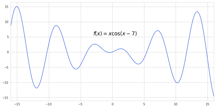
First thing to do is to pick a point from which the function will be approximated - the centering point. It would look easier if we take this point where $x$ equals zero. Taylor series approximated at point zero are also called Maclaurin series.

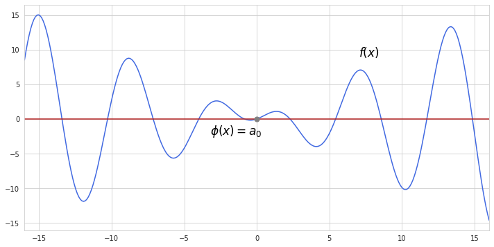
Now how do we construct a polynomial by using a single point? Firstly, we can adjust a constant term of a function by making it pass through our selected point. A constant term is just a horizontal line which needs to be fitted to our point where $x$ equals zero. In our example this constant is also zero, and it will be the starting point for fitting the approximated function $\phi(x)$ to the actual function $f(x)$.

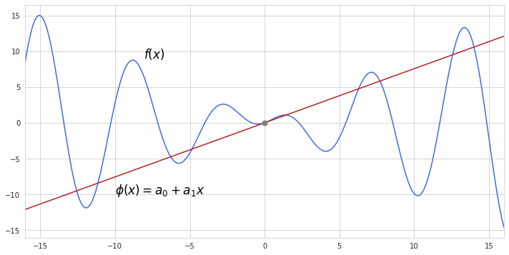
Not a very good approximation so far, right? We can do better. Recall that the derivative of a function represents its slope. By taking the derivative $f’(0)$ we can get a slope of $f(x)$ at the centering point, which we can further use in estimating the slope of the approximation function $\phi(x)$. Now, in order to add this slope to $\phi(x)$ we add to the constant term a first degree polynomial with such coefficient $a_1$ which will ensure having the same derivative as $f(x)$ at the centering point. Since we are building a first degree polynomial, its derivative is equal to the coefficient at $x$, which means $a_1$ equals to $f’(0)$. Here is how the approximation function looks now, after the we include the slope of $f(x)$ at the centering point:

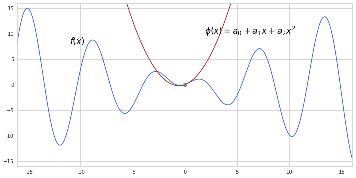
This fit is better but terrible still. We can do more by including higher order derivatives of $f(x)$. After calculating $f’’ (0)$ adding a new polynomial term to $\phi(x)$ would also require slight adjustments to $a_2$. Since the derivative of quadratic term produces $2x$ we should multiply $f’’ (0)$ by $\frac{1}{2}$ so that $\phi’’ (x)$ will have the same value as $f’’ (x)$ at the centering point. As we see, by including the second degree polynomial we made our function “curve” better around the centering point.

Since higher degree polynomials produce additional coefficients after taking derivatives of them, including more polynomial terms into the approximation function will also require additional adjusting multiplications of the terms as we explicitly did for quadratic function. The general formula for this process will look like this:

     $\phi(x) = f(0) + f’(0)\frac{x^1}{1!} + f’’ (0)\frac{x^2}{2!} + f’’’ (0)\frac{x^3}{3!} + …$

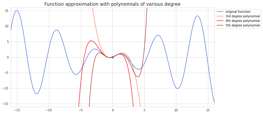
Adding more terms will make approximation around the centering point even better but at a lesser rate each time. Below is what $\phi(x)$ will look like if we include further polynomial terms.

This whole example was done using the Maclaurin series with centering point at zero. More general Taylor approximation allows selection of any point for centering approximation function. Here is the equation for Taylor series:

     $\sum_{n=0}^{\infty}\frac{f^{(n)}(a)}{n!}(x-a)^n$,

where $a$ is the centering point.