Differential equations
Differential equation is an equation with a function and at least one of its derivatives. Here is an example:
$f’’ (x) + 2f’(x) = 3f(x)$
The solution for a differential equation is a function or a set of functions, since there is often more than one solution. For the example equation above there is a solution $y_1=e^{-3x}$. The first and the second derivatives of this function would look as follows:
$y_1’ = -3e^{-3x}$,
$y_1’’ = 9e^{-3x}$
If we put these values into the original equation we can verify that indeed the function $y_1=e^{-3x}$ is the solution of the equation. This, however, is not the only solution. For example the function $y_2=e^x$ also fits to the equation.
Modeling with differential equations
Differential equations are very useful in modeling and simulation of different phenomena.
Exponetial models
Exponential models are used in modeling continuous growth or decay. It occurs when the instantaneous rate of change (that is, the derivative) of a quantity with respect to time is proportional to the quantity itself. Examples include growth of bacteria, nuclear chain reaction, radioactive decay, and economic growth expressed in percentage terms.
Here is a simple example of modeling number of users of a certain social network, such as Instagram or Facebook.
Let’s define $N$ as number of users and $t$ as time. It would be reasonable to say that the rate of change in users with respect to time is proportional to the current number of users: we assume that the actual users are sharing their experiences among their friends and so attracting new users to the network. This is how the equation will look like:
$\frac{dN}{dt}=rN$,
where $r$ is the coefficient, which may represent the number of new users each existing user is bringing into network, in other words the rate of growth.
We may recognize that this is a separable differential equation. Let’s find the solution by transforming it and using integration:
$\frac{dN}{N}=rdt \rightarrow \int\frac{dN}{N}=\int rdt \rightarrow \ln (\lvert N \rvert)=rt+C \rightarrow N=e^{rt}e^{C}=Ce^{rt}$,
where $C$ is some constant.
At the end we got the traditional form of exponential equation.
Let’s also take a closer look at $C$ value. What the value of $N$ would be if $t=0$:
$N(t=0)=Ce^{0}=C \rightarrow C=N_0$
So $C$ is basically the starting point of exponential equation.
As unbounded growth in real life is hardly possible, exponential growth models can be applied only to certain limited regions. Although growth may initially be exponential, the modelled phenomena will eventually enter a region in which previously ignored negative feedback factors become significant (leading to a logistic growth model) or other underlying assumptions of the exponential growth model, such as continuity or instantaneous feedback, break down.
Logistic models
Considering that constant exponential growth is hardly possible, logistic models assume that a function can reach only a certain level of growth. Consider the example below:
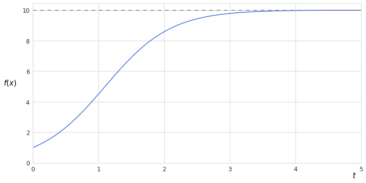
At first we see the growth is similar to exponential, however, it becomes insignificant when the function reaches its asymptote. The function cannot exceed a certain value, which in practice can be explained by the maximum capacity of the environment. For example, the population of bacteria which increases exponentially remains constant after the amount of resources in the environment becomes scarce. At this point existing individuals start competing among themselves for the resources and the growth ceases whereas the whole number of population remains at level which allows scarcity of the resources.
The differential equation for logistic models is similar to the one of exponential models but it additionally includes the hampering factor of existing population with regard to the maximum value of the function:
$\frac{dN}{dt}=rN(1-\frac{N}{K})$,
where $K$ is carrying capacity, that is the maximum possible value of a function.
The solution to this differential equation is the following function:
$N=\frac{K}{1+(\frac{K-N_0}{N_0})e^{-rt}}$