Analyzing functions

Given an equation, understanding of derivatives allows analyzing functions beyond simple plotting and eyeballing them. Below I will describe some of the techniques which can be applied in the analysis.

Finding critical values

According to the extreme value theorem, if a function is continuos at a closed interval [a, b] then this function must attain absolute minimum and maximum at least once over that interval. Let’s consider the example below:

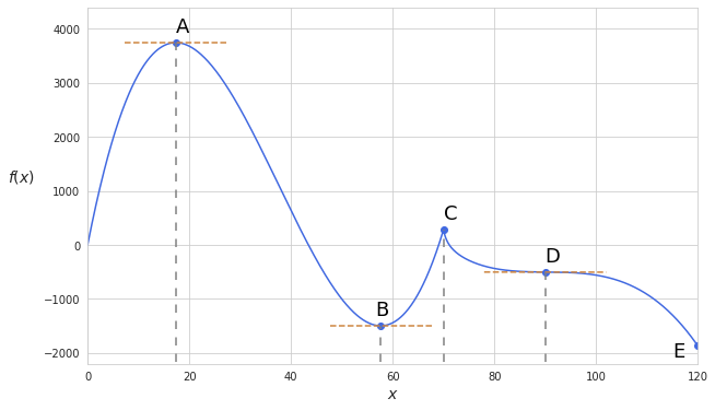
Let’s assume that the function keeps getting lower if $x$ becomes negative and if $x$ becomes greater than 120. So what is the maximum of this function? By simple eyeballing we can see that the maximum is at point A. Since the function values only keep getting lower beyond the scope of the graph, point A is the global maximum of the function. As for the global minimum, there is none since the function goes to infinity in both directions. Yet, at the end of this closed interval at the point E we have an absolute minimum where the function reaches its lowest value.

At point B we can see local minimum. One way of understanding the local minimum is that $f(x)$ assumes greater values if $x$ goes in any direction from its current value; the value of a function at a point of local minimum is relatively smaller than any of its neighboring points. Similarly, the same logic applies to the local maximum at point C.

Now when we identified all the points of maximum and minimum let’s look at the derivative of the function at those points. We see that the slope at points A and B reaches zero ($f’(x)=0$) and the tangent line goes parallel to the x-axis. As for the point C, the function is not differentiable there and the slope cannot be defined, so $f’(x)$ at that particular point does not exist. As we see, the points of maxima and minima of a function are at the points where $f’(x)=0$ or $f’(x)$ is undefined. Such points are called critical points. Looking at the graph we also see that at point D $f’(x)$ also equals to 0, so is this also a critical point? Well, yes. Although point D is neither local minimum or local maximum (generally called saddle point).

So here is the definition of critical number: $c$ is a critical value of a function $f(x)$ only if $f’(x) = 0$ or $f’(x)$ is undefined.

So basically if we want to find local minimum and maximum values of a function we need to inspect its critical values. But how do we know if a critical value is local minimum or maximum (or neither)? After looking at the graph in our example it is clear that we get local maximum if the derivative of a function was positive before reaching the critical point and became negativa afterwards. Similar logic applies for determining local minimum.

If we want to find absolute minimum and maximum values over a closed interval we need to inspect its critical values AND its closing points since the function may reach more extreme values beyond its critical points.

Finding increasing or decreasing interval

Suppose we have a function $f(x) = x^6-3x^5$.
The function is decreasing over the ponts where its derivative is less then 0. The derivative of the function looks like this: $f’(x)=6x^5-15x^4$.
The derive can be further decomposed to this form: $3x^4(2x-5)$. Given that this equation has to be less than 0 we have the following inequalities:

\[\begin{cases} 3x^4 > 0 \\ 22x-5 < 0 \end{cases}\]

or

\[\begin{cases} 3x^4 < 0 \\ 22x-5 > 0 \end{cases}\]

At the end we arrive at the solution with the interval $x<0$ or $0<x<\frac{5}{2}$ where the rate of change of the function is negative. Therefore, this is the interval where $f(x)$ is decreasing as $x$ is increasing.

Concavity of a function

Now that we know how to identify points of minima and maxima of a function using its derivative, we can move on to understanding concavity of a function. Let’s look at the example below where I plotted a function, its derivative and its second derivative:

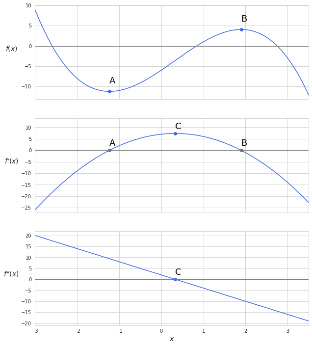
So we see that the function reaches its local minimum and maximum at points A and B respectively. At the same time we notice that the function is concave upwards around the point of local minimum and downwards around the point of local maximum. The values of the derivative of the function move upwards towards point C becoming positive after reaching point A. Namely the change from negative to positive of the derivative implies that the function reached its local minima.

By plotting second derivative we see that it is positive before point C and negative afterward. Being the derivative of the derivative function we see that point C is the critical value of the first derivative. So what this all tells us is that the rate of change of the derivative function increases all the way to the point C and then starts to decrease. As for the original function, we see that it is concave upwards at the region where its rate of change increases (or the second derivative is higher than 0) and, accordingly, concave downwards when the rate of change decreases (or the second derivative is lower than 0).

While first derivative shows the rate of change, second derivative represents acceleration. Here is one intuitive explanation of concavity with regard to acceleration:

• when acceleration is positive the function shows upwards concavity; $f(x)$ changes at greater steps than $x$;
• when acceleration is negative the function shows downwards concavity; $f(x)$ changes at lesser steps than $x$.

Meanwhile, we see that at the points of local minimum and maximum first derivatives are equal to 0 however their corresponding second derivatives are greater or lesser than 0. Therefore, in order to know if the critical point is minimum or maximum we do not need to calculate the derivatives of neighbouring values to the critical point. We can simply take the second derivative and draw conclusions from there. If at the critical point the second derivative is greater than zero then we have a point of local minimum, same logic applies to recognizing the point of local maximum.